![]()
Machine Learning with scikit-learn
Andreas Mueller
Overview
- Basic concepts of machine learning
- Introduction to scikit-learn
- Some useful algorithms
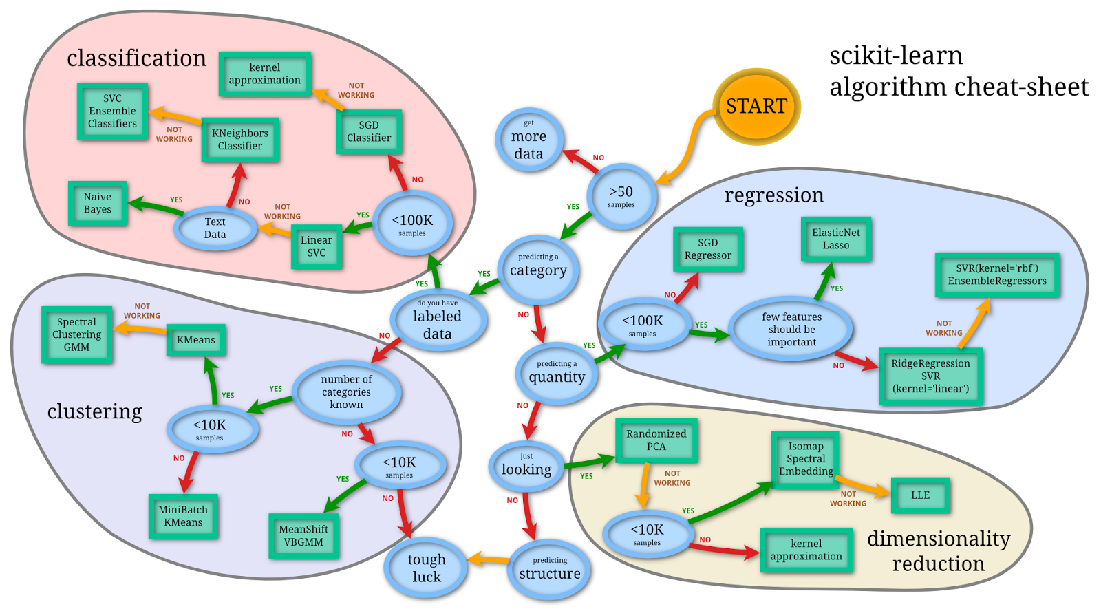
- Selecting a model
- Working with text data
scikit-learn
- Collection of machine learning algorithms and tools in Python.
- BSD Licensed, used in academia and industry (Spotify, bit.ly, Evernote).
- ~20 core developers.
- Take pride in good code and documentation.
- We want YOU to participate!
Two (three) kinds of learning
- Supervised
- Unsupervised
- Reinforcement
Supervised learning
Training: Examples X_train together with labels y_train.
Testing: Given X_test, predict y_test.
Examples
- Classification (spam, sentiment analysis, ...)
- Regression (stocks, sales, ...)
- Ranking (retrieval, search, ...)
Unsupervised Learning
Examples X. Learn something about X.
Examples
- Dimensionality reduction
- Clustering
- Manifold learning
Data representation
Everything is a numpy array (or a scipy sparse matrix)!
Let's get some toy data.
from sklearn.datasets import load_digits
digits = load_digits()
print("images shape: %s" % str(digits.images.shape))
print("targets shape: %s" % str(digits.target.shape))
plt.matshow(digits.images[0], cmap=plt.cm.Greys);

digits.target
Prepare the data
X = digits.data.reshape(-1, 64)
print(X.shape)
y = digits.target
print(y.shape)
We have 1797 data points, each an 8x8 image -> 64 dimensional vector.
X.shape is always (n_samples, n_feature)
print(X)
Taking a Peek
Dimensionality Reduction and Manifold Learning
- Always first have a look at your data!
- Projecting to two dimensions is the easiest way.
Principal Component Analysis (PCA)
from sklearn.decomposition import PCA
Instantiate the model. Set parameters.
pca = PCA(n_components=2)
Fit the model.
pca.fit(X);
Apply the model. For embeddings / decompositions, this is transform.
X_pca = pca.transform(X)
X_pca.shape
plt.figsize(16, 10)
plt.scatter(X_pca[:, 0], X_pca[:, 1], c=y);

print(pca.mean_.shape)
print(pca.components_.shape)
fix, ax = plt.subplots(1, 3)
ax[0].matshow(pca.mean_.reshape(8, 8), cmap=plt.cm.Greys)
ax[1].matshow(pca.components_[0, :].reshape(8, 8), cmap=plt.cm.Greys)
ax[2].matshow(pca.components_[1, :].reshape(8, 8), cmap=plt.cm.Greys);

Isomap
from sklearn.manifold import Isomap
Instantiate the model. Set parameters.
isomap = Isomap(n_components=2, n_neighbors=20)
Fit the model.
isomap.fit(X);
Apply the model.
X_isomap = isomap.transform(X)
X_isomap.shape
plt.scatter(X_isomap[:, 0], X_isomap[:, 1], c=y);

Classification
To evaluate the algorithm, split data into training and testing part.
from sklearn.cross_validation import train_test_split
X_train, X_test, y_train, y_test = train_test_split(X, y, random_state=0)
print("X_train shape: %s" % repr(X_train.shape))
print("y_train shape: %s" % repr(y_train.shape))
print("X_test shape: %s" % repr(X_test.shape))
print("y_test shape: %s" % repr(y_test.shape))
Start Simple: Linear SVMs
from sklearn.svm import LinearSVC
Finds a linear separation between the classes.
Instantiate the model.
svm = LinearSVC()
Fit the model using the known labels.
svm.fit(X_train, y_train);
Apply the model. For supervised algorithms, this is predict.
svm.predict(X_train)
Evaluate the model.
svm.score(X_train, y_train)
svm.score(X_test, y_test)
More complex: Random Forests
from sklearn.ensemble import RandomForestClassifier
Builds many randomized decision trees and averages their results.
Instantiate the model.
rf = RandomForestClassifier()
Fit the model.
rf.fit(X_train, y_train);
Evaluate.
rf.score(X_train, y_train)
rf.score(X_test, y_test)
Model Selection and Evaluation
Always keep a separate test set to the end.
- Measure performance using cross-validation
from sklearn.cross_validation import cross_val_score
scores =  cross_val_score(rf, X_train, y_train, cv=5)
print("scores: %s  mean: %f  std: %f" % (str(scores), np.mean(scores), np.std(scores)))
Maybe more trees will help?
rf2 = RandomForestClassifier(n_estimators=50)
scores =  cross_val_score(rf2, X_train, y_train, cv=5)
print("scores: %s  mean: %f  std: %f" % (str(scores), np.mean(scores), np.std(scores)))
Adjust important parameters using grid search
from sklearn.grid_search import GridSearchCV
- Let's look at LinearSVC again.
- Only important parameter: C
param_grid = {'C': 10. ** np.arange(-3, 4)}
grid_search = GridSearchCV(svm, param_grid=param_grid, cv=3, verbose=3, compute_training_score=True)
grid_search.fit(X_train, y_train);
print(grid_search.best_params_)
print(grid_search.best_score_)
plt.figsize(12, 6)
plt.plot([c.mean_validation_score for c in grid_search.cv_scores_], label="validation error")
plt.plot([c.mean_training_score for c in grid_search.cv_scores_], label="training error")
plt.xticks(np.arange(6), param_grid['C']); plt.xlabel("C"); plt.ylabel("Accuracy");plt.legend(loc='best');

Overfitting and Complexity Control
-
to the right: overfitting aka high variance.
- Means no generalization.
-
to the left: underfitting aka high bias.
- Means bad even on training set.
plt.plot([c.mean_validation_score for c in grid_search.cv_scores_], label="validation error")
plt.plot([c.mean_training_score for c in grid_search.cv_scores_], label="training error")
plt.xticks(np.arange(6), param_grid['C']); plt.xlabel("C"); plt.ylabel("Accuracy");plt.legend(loc='best');
Detecting Insults in Social Commentary
- My first (and only) kaggle entry.
- Classify short forum posts as insulting or not.
- A simple bag of word model carries quite far.
- Linear classifiers are usually the best for text data.
Read the CSV using Pandas (a bit overkill).
import pandas as pd
train_data = pd.read_csv("kaggle_insult/train.csv")
test_data = pd.read_csv("kaggle_insult/test_with_solutions.csv")
- The column "Insult" contains the target.
- The column "Comment" contains the text.
y_train = np.array(train_data.Insult)
comments_train = np.array(train_data.Comment)
print(comments_train.shape)
print(y_train.shape)
print(comments_train[0])
print("Insult: %d" % y_train[0])
print(comments_train[5])
print("Insult: %d" % y_train[5])
Vectorizing the Data
from sklearn.feature_extraction.text import CountVectorizer
- Use bag of words model as implemented in CountVectorizer.
- Extracts a dictionary, then counts word occurences.
cv = CountVectorizer()
cv.fit(comments_train)
print(cv.get_feature_names()[:15])
print(cv.get_feature_names()[1000:1015])
X_train = cv.transform(comments_train).tocsr()
print("X_train.shape: %s" % str(X_train.shape))
print(X_train[0, :])
Training a Classifier
- LinearSVC : linear SVM that is efficient for sparse data.
from sklearn.svm import LinearSVC
svm = LinearSVC()
svm.fit(X_train, y_train)
comments_test = np.array(test_data.Comment)
y_test = np.array(test_data.Insult)
X_test = cv.transform(comments_test)
svm.score(X_test, y_test)
print(comments_test[8])
print("Target: %d, prediction: %d" % (y_test[8], svm.predict(X_test.tocsr()[8])[0]))
Next Steps
- Grid search
Cparameter of LinearSVC.
- Build a pipeline, adjust parameters of feature extraction.
- Combine different feature extraction methods.
Take Away
- Get your data into an array
(n_samples, n_features).
- model.fit(X), model.predict(X) / model.transform(X)
- Always do cross-validation. Leave the test set until the end.
- Internalize the complexity / generalization tradeoff.
Fin
| amueller@ais.uni-bonn.de | |
| @t3kcit | |
 | @amueller |
| peekaboo-vision.blogspot.com |