Introduction
This book aims to provide an accessible introduction into applying machine learning with Python, in particular using the scikit-learn library. I assume that you’re already somewhat familiar with Python and the libaries of the scientific Python ecosystem. If you find that you have a hard time following along some of the details of numpy, matplotlib and pandas, I highly recommend you look at Jake VanderPlas’ Python Data Science handbook.
Scope and Goals
After reading this book, you will be able to do exploratory data analysis on a dataset, evaluate potential machine learning solutions, implement, and evaluate them. The focus of the book is on tried-and-true methodology for solving real-world machine learning problems. However, we will not go into the details of productionizing and deloying the solutions. We will mostly focus on what’s know as tabular data, i.e. data that would usually be represented as a pandas DataFrame, Excel Spreadsheet, or CSV file. While we will discuss working with text-data in Chapter, there are many more advanced techniques, for which I’ll point you towards Dive into Deep Learning by Aston Zhang, Zachary C. Lipton, Mu Li, and Alexander J. Smola. We will not look at image recognition, video or speech data, or time series forecasting, though many of the core concepts described in this book will also apply there.
What is machine learning?
Machine learning, also known as predictive modeling in statistics, is a research field and a collection of techniques to extract knowledge from data, often used to automate decision-making processes. Applications of machine learning are pervasive in technology, in particular in complex websites such as facebook, Amazon, youtube or Google. These sites use machine learning to personalize the experience, show relevant content, decide on advertisements, and much more. Without machine learning, none of these services would look anything like they do today. Outside the web, machine learning has also become integral to commercial applications in manifacturing, logistics, material design, financial markets and many more. Finally, over the last years, machine learning has also become essential to research in practically all data-driven sciences, including physics, astronomy, biology, medicine, earth sciences and social sciences.
There are three main sub-areas of machine learning, supervised learning, unsupervised learning, and reinforcement learning, each of which applies to a somewhat different setting. We’ll discuss each in turn, and give some examples of how they can be used.
Supervised Learning
Supervised learning is by far the most commonly used in practice. In supervised learning, a model is built from a dataset of input-output pairs, where the input is known as features or independent variables, which we’ll denote by \(x\), and the output is known as target or label, which we’ll denote by \(y\). The input here is a representation of an entity of interest, say a customer to your online shop, represented by their age, location and shopping history. The output is a quantity of interest that we want our model to predict, say whether they would buy a particular product if we recommend it to them. To build a model, we need to collect many such pair, i.e. we need to build records of many customers and their decisions about whether or not they bought the product after an recommendation was shown to them. Such a set of input-output pairs for the purpose of building a supervised machine learning model is called a training set.
Once we collected this dataset, we can (attempt to) build a supervised machine learning model that will make a prediction for a new user that wasn’t included in the training dataset. That might enable us to make better recommendations, i.e. only show recommendations to a user that’s likely to buy.
The name supervised learning comes from the fact that during learning, the dataset contains the correct targets, which acts as a supervisor for the model training.
For both regression and classification, it’s important to keep in mind the concept of generalization. Let’s say we have a regression task. We have features, that is data vectors x_i and targets y_i drawn from a joint distribution. We now want to learn a function f, such that f(x) is approximately y, not on this training data, but on new data drawn from this distribution. This is what’s called generalization, and this is a core distinction to function approximation. In principle we don’t care about how well we do on x_i, we only care how well we do on new samples from the distribution. We’ll go into much more detail about generalization in about a week, when we dive into supervised learning.
Classification and Regression
There are two main kinds of supervised learning tasks, called classification and regression\(^1\). If the target of interest \(y\) that we want to predict is a quantity, the task is a regression problem. If it is discrete, i.e. one of several distinct choices, then it is a classification problem. For example, predicting the time it will take a patient to recover from an illness is a regression task, say measured in days. We might want our model to predict whether a patient will be ready to leave a hospital 3.5 days after admission or 5 or 10. This is regression becaues the time is clearly a continuous quantity, and there is a clear sense of ordering and distance between the different possible predictions. If the correct prediction is that the patient can leave after 4.5 days, but instead we predict 5, that might not be exactly correct, but it might still be a useful prediction. Even 6 might be somewhat useful, while 20 would be totally wrong.
An example for a classification task would be which of a set of medications the patient would respond best to\(^2\). Here, we have a fixed set of disjoint candidates that are known a-priori, and there is usually no order or sense of distance between the classes. If medication A is the best, then predicting any other medication is a mistake, so we need to predict the exact right outcome for the prediction to be accurate. A very common instance of classification is the special case of binary classification, where there are exactly two choices. Often this can be formulated as a “yes/no” question to which you want to predict an answer. Examples of this are “is this email spam?”, “is there a pedestrian on the street”, “will this customer buy this product” or “should we run an X-ray on this patient”.
The distinction into classification is important, as it will change the algorithms we will use, and the way we measure success. For classification, a common metric is accuracy, the fraction of correctly classified examples, i.e. the fraction of times the model predictied the right class. For regression on the other hand, a common metric is mean squared error, which is the squared average distance from the prediction to the correct answer. In other words, in regression, you want the prediction to be close to the truth, while in classification you want to predict exactly the correct class. In practice, the difference is a bit more subtle, and we will discuss model evaluation in depth in chapter TODO.
Usually it’s quite clear whether a task is classification or regression, but there are some cases that could be solved using either approach. A somewhat common example is ratings in the 5-star rating system that that’s popular on many online platforms. Here, the possible ratings are one start, two starts, three stars, four stars and five stars. So these are discrete choices, and you could apply a classification algorithm. On the other hand, there is a clear ordering, and if the real answer is one star, predicting two stars is probably better than predicting 5 stars, which means it might be more appropriate to use regression. Here, which one is more appropriate depends on the particular algorithm you’re using and how to integrate into your larger workflow.
Generalization
When building a model for classification or regression, keep in mind that what we’re interested in is applying the model to new data for which we do not know the outcome. If we build a model for detecting spam emails, but it only works on emails in the training set, i.e. emails the model has seen during building of the model, it will be quite useless. What we want from a spam detection algorithm is to predict reasonably well whether an email is spam or not for a new email that was not included in the training set. The ability for a supervised model to make accurate predictions on new data is called generalization and is the core goal of supervised learning. Whithout asking for generalization, an algorithm could solve the spam detection task on the training data by just storing all the data, and when presented with one of these emails, look up what the correct answer was. This approach is known as memorization, but it’s impossible to apply to new data.
Conditions for success
For a supervised learning model to generalize well, i.e. for it to be able to learn to make accurate prediction on new data, some key assumptions must be met:
First, the necessary information for making the correct prediction actually needs to be encoded in the training data. For example, if I try to learn to predict a fair coin flip before the coin is tossed, iI won’t be able to build a working machine learning model, no matter what I choose as the input features. The process is very (or entirely?) random, and the information to make a prediction is just not available. More technically, one might say the process has high intrinsic randomness that we can not overcome by building better models. While you’re unlikely to encounter a case as extreme (and obvious) as a coin toss, many processes in the real world are quite random (such as the behavior of people) and it’s impossible to make entirely accurate predictions for them.
In other cases, a prediction might be possible in principle, but we might not have provided the right information to the model. For example, it might be possible for a machine learning model to learn to diagnose pneumonia in a patient, but not if the only information about the patient that we represent to them is their shopping habbits and wardrobe. If we use a chest x-ray as a representation of the patient, together with a collection of symptoms, we will likely have better success. Even if the information is represented in the input, learning might still fail if the model is unable to extract the information. For example, visual stimuli are very easy to interpret for humans, but in general much harder to understand for machine learning algorithms. Consequently, it would be much harder for a machine to determine if a graffiti is offensive by presenting it with a photograph, than if the same information was represented as a text file.
Secondly, the training dataset needs to be large and varied enough to capture the variability of the process. In other words, the training data needs to be representative of the whole process, not only representing a small portion of it. Humans are very good at abstracting properties, and a child will be able to understand what a car is after seeing only a handfull. Machine learning algorithms on the other hand require a lot of variability to be present. For example, to learn the concept of what a car looks like, an algorithm likely needs to see pictures of vans, of trucks, of sedans, pictures from the front, the side and above, pictures parking and in traffic, pictures in rain and in sunshine, in a garage and outdoors, maybe even pictures taken by a phone camera and pictures taken by a news camera. As we said before, the whole point of supervised learning is to generalize, so we want our model to apply to new settings. However, how new a setting can be depends on the representation of the data and the algorithm in question. If the algorithm has only ever seen trucks, it might not recognize a sedan. If the algorithm has never seen a snow-covered car, it’s unlikely it will recognize it. Photos (also known as natural images in machine learning) are a very extreme example as they have a lot of variability, and so often require a lot of training data. If your data has a simple structure, or the relationship between your features and your target are simple, then only a handful of training examples might be enough.
Third and finally, the data that the model is applied to needs to be generated from the same process as the data the model was trained on. A model can only generalize to data that in essence adheres to the same rules and has the same structure. If I collect data about public transit ridership in Berlin, and use it to make predictions in New York, my model is likely to perform poorly. While I might be able to measure the same things, say number of people at stations, population density, holidays etc, there are so many differences between data collected in Berlin and data collected in New York that it’s unlikely a model trained on one could predict well on the other. As another example, let’s say you train an image recognition model for recognizing hot dogs on a dataset of stock photos, and you want to deploy it to an app using a phone camera. This is also likely to fail, as stock photography doesn’t resemble photos taken by users pointing their phone. Stock photography is professionally produced and well-lit, the angles are carefully chosen, and often the food is altered to show it in it’s best light (have you noticed how food in a restaurant never looks like in a commercial?). However, machine learning requires you to use a training dataset that was generated by the same process as the data the model will be applied to.
Mathematical Background
From a mathematical standpoint, supervised learning assumes that there is a joint distribution \(p(x, y)\) and that the training dataset consists for independent, identically distributed (i.i.d.) samples from this joint distribution. The model is then applied to new data sampled from the same distribution, but \(y\) is unknown. The model is then used to estimate \(p(y | x)\), or more commonly the mode of this distribution, i.e. the most likely value for \(y\) to take given the \(x\) we observed. In the case of learning to predict a coin flip, you could actually learn a very accurate model of \(p(y | x)\), that predicts heads and tails with equal probability. There is no way to predict the particular outcome itself, though.
The third requirement for success is easily expressed as saying that the test data is sampled i.i.d. from the same distribution \(p(x, y)\) that the training data was generated from.
Unsupervised Learning
In unsupervised machine learning, we are usually just given data points \(x\), and the goal is to learn something about the structure of the data. This is usually a more open-ended task than what we saw in supervised learning. This kind of task is called unsupervised, because even during training, there is no “supervision” providing a correct answer. There are several sub-categories of unsupervised learning that we’ll discuss in Chapter 3, in particular clustering, dimensionality reduction, and signal decomposition. Clustering is the task of finding coherent groups within a dataset, say subgroups of customers that behave in a similar way, say “students”, “new parents” and “retirees”, that each have a distinct shopping pattern. However, here, in contrast to classification, the groups are not pre-defined. We might not know what the groups are, how many groups there are, or even if there is a coherent way to define any groups. There might also be several different ways the data could be grouped: say you’re looking at portraits. One way to group them could be by whether the subject has classes or not. Another way to group them could be by the direction they are facing. Yet another might be hair color or skin color. If you tell an algorithm to cluster the data, you don’t know which aspect it will pick up on, and usually manually inspecting the groups or clusters is the only way to interpret the results.
Two other, related, unsupervised learning tasks are dimensionality reduction and signal decomposition. In these, we are not looking at groups in the data, but underlying factors of variance, that are potentially more semantic than the original representation. Going back to the example of portraits, an algorithm might find that head orientation, lighting and hair color are important aspects of the image that vary independently. In dimensionality reduction, we are usually looking for a representation that is lower-dimensional, i.e. that has less variables than the original feature space. This can be particularly useful for visualizing dataset with many features, by projecting them into a two-dimensional space that’s easily plotted. Another common application of signal decomposition is topic modeling of text data. Here, we are trying to find topics among a set of documents, say news articles, or court documents, or social media posts. This is related to clustering, though with the difference that each document can be assigned multiple topics, i.e. topics in the news could be politics, religion, sports and economics, and an article could be about both, politics and economics.
Both, clustering and signal decomposition, are most commonly used in exploratory analysis, where we are trying to understand the data. They are less commonly used in production systems, as they lend themselves less easily to automating a decision process. Sometimes signal decomposition is used as a mechanism to extract more semantic features from a dataset, on top of which a supervised model is learned. This can be particularly useful if there is a large amount of data, but only a small amount of annotated data, i.e. data for which the outcome \(y\) is known.
Reinforcement Learning
The third main family of machine learning tasks is reinforcement learning, which is quite different from the other two. Both supervised and unsupervised learning basically work on a dataset that was collected and stored, from which we then build a model. Potentially, this model is then applied to new data in the future. In reinforcement learning, on the other hand, there is no real notion of a dataset. Instead, reinforcement learning is about a program (usually known as an agent) interacting with a particular environment. Through this interaction, the agent learns to achieve a particular goal. A good example of this is a program learning to play a video game. Here, the agent would be an AI playing the game, while the environment would be the game itself, i.e. the world in which it plays out. The agent is presented with the environment, and has choices of actions (say moving forward and backward and jumping) and each of these actions will result in the environment being in a new state (i.e. with the agent placed a bit forward, or backward, or falling in a hole). Given the new environment, the agent again can choose an action and the environment will be in a new state as a consequence.
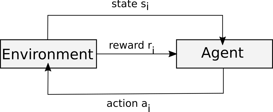
Fig. 1 The reinforcement learning cycle.
The learning in reinforcement learning happens with so-called rewards, which need to be specified by the data scientist building the system. The agent is trained to seek rewards (hence the name reinforcement learning), and will find series of actions that maximize its reward. In a game, a reward could be given to the environment every time they score points, or just once when the agent wins the game. In the second case, there might be a long delay between the agent taking an action, and the agent winning the game, and one of the main challenges in reinforcement learning is dealing with such settings (this is known as credit attribution problem: which of my actions should I give credit for me winning the game).
Compared with supervised learning, reinforcement learning is a much more indirect way to specify the learning problem: we don’t provide the algorithm with the correct answer (i.e. the correct sequence of actions to win the game), instead we only reward the agent once they achieve a goal. Suprisingly, this can work surprisingly well in practice. This is like learning a game without someone ever telling you the rules, or what the goal of the game is, but only telling you whether you lost or won at the end. As you might expect, it might take you many many tries to figure out the game.
However, algorithms are notoriously patient, and researchers have been able to use reinforcement learning to create programs that can play a wide variety of complex games. Potentially one of the most suprising and impressive feats was learning to play the ancient chinese boardgame of Go at a superhuman level.
When this was publicided in TODO, many researchers in the area were shocked, as the game was known to be notoriously hard, and many believed it could not be learned by any known algorithms. While the initial work used some human knowledge, later publications learned to play the game from scratch, i.e. without any rewards other than for winning the game, by the agent repeatedly playing the game against itself. The resulting programs are now playing at superhuman level, meaning that they are basically unbeatable, even by the best human players in the world. Similar efforts are now underway for other games, in particular computer games like StarCraft II and DOTA.
Reinforcement learning also has a long history in other areas, in particular robotics, where it is used for learning and tuning behaviors, such as walking or grasping. While many impressive achievements have been made with reinforcement learning, there are several aspects that limit it’s broad usefulness. A potential application of reinforcement learning could be self-driving cars. However, as mentioned above, reinforcement learning usually requires many attempts or iterations before it learns a specific task. If I wanted to train a car to learn to park, it might fail thousands or hundreds of thousands of times first. Unfortunately, in the real world this is impractical: self-driving cars are very expensive, and we don’t want to crash them over and over again. It might also be risky for the person conducting the experiment. With thousands of attempts, even if the car doesn’t crash, the gas will run out, and the person having to reset the experiment every time will probably get very tired very quickly. Therefore, reinforcement learning is most successful when there is a good way to simulate the environment, as is the case with games, and with some aspects of robotics. For learning how to park, a simulation might actually work well, as the sensing of other cars and the steering of the car can be simulated well. However, for really learning how to drive, a car would need to be able to deal with a variety of situations, such as different weather conditions, crowded streets, people running on the strees, kids chasing balls, navigating detours and many other scenarios. Simulating these in a realistic way is very hard, and so reinforcement learning is much harder to apply in the physical world.
A setting that has attracted some attention, and might become more relevant soon, is online platforms that are not games. You could think of a social media timeline as an agent that gets rewarded for you looking at it. Right now, this is often formulated as a supervised learning task (TODO or more acurately active learning). However, your interactions with social media are not usually indepentent events, but your behavior online is shaped by what is being presented to you, and what was shown to you in the past might influence what is shown to you in the future. A maybe somewhat cynical analogy would be to think of this as a timeline being an agent, playing you, winning whenever you stay glued to the screen (or click an ad or buy a product). I’m not aware that this has been implemented anywhere, but as computational capacity increase and algorthms become more sophisticated, it is a natural direction to explore.
Reinforcement learning is a fascinating topic, but much beyond the scope of this book. For an introduction, see TODO Sutten Barto. For an overview of modern approaches, see TODO.
As you might have notices in the table of contents, this book mostly concerns itself with supervised and unsupervised learning, and we will not discuss reinforcement learning any further. As a matter of fact, the book heavily emphasizes supervised learning, which has found the larges success among the three in practical applications so far. While all three of these areas are interesting in their own right, when you see an application of machine learning, or when someone says they are using machine learning for something, chances are they mean supervised learning, which is arguably the most well-understood, and the most easy to productionize and analyze.
Isn’t this just statistics?
A very common question I get is ‘is machine learning not just statistics?’ and I want to quickly address how the approach in this book differs from the approach taken in a statistics class or textbook. The machine learning community and the statistics community have some historical differences (ML being born much later and from within computer science), but study many of the same subjects. So I don’t think it makes sense to say that one thing is statistics and the other thing is machine learning. However, there is usually a somewhat different emphasis in the kinds of problems and questions that are addressed in either, and I think it’s important to distinguish these tasks. Much of statistics often deals with inference, which means that given a dataset, we want to make statements that hold for the dataset (often called population in statistics) as a whole. Machine learning on the other hand often emphasizes prediction, which means we are looking to make statements about each sample, in other words indivdual level statements. Asking “do people that take zinc get sick less often”” is an inference question, as it asks about whether something happens on average over the whole population. A related prediction question would be “will this particular person get sick if they take zinc?”. The answer for the inference question would be either “yes” or “no”, and using hypothesis testing methodology this statement could have an effect size and a significance level attached to it. The answer for the prediction question would be a prediction for each sample of interest, or maybe even a program that can make prediction given information about a new patient.
As you can see, these are two fundamentally different kinds of questions, and require fundamentally different kinds of tools to answer them. This book solely looks at the prediction task, and we consider a model a good model if it can make good predictions. We do not claim that the model allows us to make any statistical or even causal statements that hold for the whole population, or the process that generated the dataset.
There are some other interesting differences between the kind of prediction questions studied in supervised machine learning compared to inference questions that are traditionally studied in statistics; in particular, machine learning usually assumes that we have access to data that was generated from the process we want to model, and that all samples are created equal (i.i.d.). Statistical inference usually makes no such assumptions, and instead assumes that we have some knowledge about the structure of the process that generated the data. As an example, consider predicting a presidential election outcome. As of this writing, there’s 58 past elections to learn from. For a machine learning task, this is by no means enough observations to learn from. But even worse, these samples are not created equally. The circumstances of the first election are clearly different than the will be for the next election. The economic and societal situation will be different, as will be the candidates. So really, we have no examples whatsoever from the process that we’re interested in. However, understanding all the differences to previous elections, we might still be able to make accurate forecasts using statistical modeling.
Some of my favorite machine learning textbooks are written by statisticians (the subfield is called predictive modeling), and there are certainly machine learning researchers that work on inference questions, so I think making a distinction between statistics and machine learning is not that useful. However, if you look at how a statistics textbook teaches, say, logistic regression, the intention is likely to be inference, and so the methods will be different from this book, where the emphasis is on prediction, and you should keep this in mind.
This is not to say that one is better than the other in any sense, but that it’s important to pick the right tool for the job. If you want to answer an inference question, the tools in this book are unlikely to help you, but if you want to make accurate predictions, they likely will.
The bigger picture
This book is mostly technical in nature, with an emphasis on practial programming techniques. However, there are some important guiding principles for developing machine learning solutions that are often forgotten by practitioners who find themselves deep in the technical aspects. In this section, I want to draw your attention to what I think are crucial aspects of using machine learning in applications. It might seem a bit dry for now, but I encourage you to keep these ideas in mind while working through the rest of the book, and maybe come back here in the end, once you’ve got your toes a bit wet.
The machine learning process
Any data science process, like most knowledge seeking processes, interleaves collecting evidence, making hypothesis, and validating them, as process also known as Box’s loop TODO.
I summarized how I think of this iterative process in Figure TODO.

Outside of the depicted process is the formulation of the problem, and the definition of measures, both of which are critical, but usually not part of the loop. The actual machine learning process itself starts with data collection, which might mean mining historical data, labeling data by hand, or running simulations or even performing actual physical experiments. Once the data is collected, it needs to be processed into a format suitable for machine learning, which we’ll discuss in more detail in Chapter TODO. Before building the model expoloratory data analysis and visualization are essential to form or confirm intuition on the structure of the data, to spot potential data quality issues, to select suitable candidate models, and potentially generate new features. The next step, model building, usually involves building several candidate models, tweaking them, and comparing them. Once a model is selected, it is usually evaluated first in an off-line manner, that is using already collected data.
Then, potentially it is further validated in a live setting with current data. Finally, the model is deployed into the production environment. For a web app, deployment might be deployment in the software sense: deploying a service that takes user data, runs the model, and renders some outcome on your website. For industrial applications, deployment could mean integrating your defect detection into an assembly line and discarding defect; if your model is for evaluating real-estate, deployment might mean buying highly valued properties.
This process is depicted as a circle, as deployment usually generates new data, or informs future data collection, and restarts the process. While I drew a circle, actually this is more than one loop, in fact this is a fully connected graph, where after each step, you might decide to go back to previous steps and start over, improving your model or your process. At any point, you might find data quality issue, figure out new informative ways to represent the data, or find out that your model doesn’t perform as well as you thought. Each time, you might decide to improve any of the previously taken steps. Usually there are many iterations before reaching integration and deployment for the first time, as using an unsuitable model might represent substantial risk to your project.
The rest of the book will focus on model building and evaluation, which are at the core of machine learning. However, for a successful project, all of the steps in the process are important. Formulating the problem, collecting data, and establishing success metrics are often at least as crucial as selecting the right model and tweaking it. Given the technical nature of the material presented in this book, it’s easy to lose sight of how critical all the steps of the process are. We will discuss some of these in a bit more detail now.
The role of data
Clearly the data used for building and evaluating a machine learning model are crucial ingredients. Data collection is often overlooked in machine learning education, where students usually look at fixed datasets, and the same is true for online competitions and platforms such as kaggle. However, in practice, data collection is usually part of building any machine learning application, and there is usually a choice to collect additional data, or to change the data collection. Having more data can be the difference between a model that’s not working, and a model that outperforms human judgement, in particular if you can collect data that covers the variablity that you will encounter in prediction. Sometimes it might be possible to collect additional features that make the task much easier, and selecting what data to collect is often as critical as selecting the right model. Usually it’s easier to throw away data later than to add new fields to the data collection. It’s common for data scientist to start working on a model only to discover that a critical aspect of the process was not logged, and a task that could have been easy becomes extremely hard.
Depending on the problem you’re tackling, the effort and cost of data collection can vary widely. In some settings, the data is basically free and endless. Say you want to predict how much attention a post will receive on social media. As long as your post is similar to other posts on the platform, you can obtain arbitrary amounts of training data by looking at existing posts, and collect the number of likes and comments and other engagement. This data rich situation often appears when you are tying to predict the future, and you can observe the labels of past data simply by waiting, i.e. seeing how many people like a photo. In some cases the same might be true for showing ads or recommendations, where you are able to observe past behavior of users, or in content moderation, where users might flag offending content for you. This assumes that the feedback loop is relatively small and the events repeat often, though. If you work in retail, the two data points that are most crucial (at least in the US) are Black Friday and Christmas. And while you might be able to observe them, you can only observe them once a year, and if you make a bad decision, you might go out of business before observing them again.
Another common situation is automating a business process that before has been done manually. Usually collecting the answers is not free in this setting, but it’s often possible to collect additional data by manually annotation. The price of collecting more data then depends on the level of qualification required to create accurate labels, and the time involved. If you want to detect personal attacks in your online community, you can likely use a crowd-sourcing platform or a contractor to get reasonable labels. If your decision requires expert knowledge, say, which period a painting was created in, hiring an expert might be much more expensive or even impossible. In this situation, it’s often intersting to ask yourself what is more cost-effective: spending time building and tuning a complex machine learning model, or collecting more data and potentially getting results with less effort. We will discuss how to make this decision in TODO.
Finally, there are situations where getting additional data is infeasible or impossible; in this situations, people speak of precious data. Examples of this could be the outcome of a drug-trial, which is lengthy and expensive and where collecting additional data might not be feasible. Or the simulation of a complex physical system, or observations on a scientific measurement. Maybe each sample corresponds to a new microchip architecture for which you want to model energy efficiency. These settings are those where tweaking your model and diving deep into the problem might pay off, but these situations are overall rather rare in practice.
Feedback loops in data collection
One particular aspect that is often neglected in data collection is that the effect of deploying a machine learning model might change the process generating the data. A simple example for this would be a spammer, who, once a model is able to flag their content, would change their strategy or content so as to be no longer detected. Clearly, the data here changed as a consequence of deploying the model, and the model that might have been able to accurately identify spam in an offline setting might not work in practice. In this example, there is an adverserial intent and the spammers intentionally try to defeat the model. However, similar changes might happen indicentally, but still invalidate a previous model. For example, when building systems for product recommentation, the model often relies on data that was collected using some other recommendation scheme, and the choice of this scheme clearly influences what data will be collected. If a streaming platform never suggests a particular movie, it’s unlikely to be seen by many users, and so it will not show up in user data that’s collected, and so a machine learning algorithm will not recommend it, creating a feedback loop that will lead to the movie being ignored. There is a whole subset of machine learning devoted to this kind of interactive data collection, called active learning, where the data that is collected is closely related to the model that’s being build. This area also has a close relation to reinforcement learning.
Given the existence of these feedback loops, it’s important to ensure that your model performs well, not only in an offline test, but also in a production environment. Often this is hard to simulate, as you might not be able to anticipate the reaction of your users to deploying an algorithm. In this case, using A/B testing might be a way to evaluate your system more rigourously.
A particular nefarious example of this feedback loop has been observed (TODO citation) in what is known as predictive policing. The premise of predictive policing is to send police patrols to neighborhoods where they expect to observe crime, at times that they expect to observe crime. However, if police is sent to a neighborhood, they are likely to find criminal activity there (even if it might be minor); and clearly they will not find criminal activity in neighborhoods they did not patrol. Historically, police patrols in certain US cities have focused on non-white neighborhoods, and given this historical data, predictive policing methods steered patrols to these same neighborhoods. Which then lead them to observe more crime there, leading to more data showing crime in these neighborhoods, leading to more patrols being send there, and so on.
Metrics and evaluation
One of the most important parts of machine learning is defining the goal, and defining a way to measure that goal. The first part of this is having the right data for evaluating your model, data that will reflect the way the model will be used in production. Equally important is establishing a measure of impact for your task. Usually your application is driven by some ultimate goal, such as user engagement, revenue, keeping patients healthy or any number of possible motivations. The question is now how your machine learning solution will impact this goal. It’s important to note that the goal is rarely if ever to make accurate predictions. It’s not some evaluation metrics that counts, but it’s the real world impact of the decision that are made by your model.
There are some common hurdles in measuring the impact of your model. Often, the effect on the bottom line might only be very indirect. If you’re removing fake news from your social media platform, this will not directly increase your ad revenue, and removing a particular fake news article will probably have no measurable impact. However, curating your platform will help maintain a brand image and might drive users to your platform, which in turn will create more revenue. But this effect is likely to be mixed in with many other effects, and much delayed in time. So often data scientists rely on surrogate metrics, measures that relate to intermediate business goals\(^3\) that can be measured more directly, such as user engagement or click-through-rate.
The problem with such surrogate metrics is that they might not capture what you assume they capture. I heard an (if not true, then at least illustrative) anectote about optimizing the placement of an ad on a shopping website. An opptimization algorithm placed it right next to the search button, with the same color as the search button, which resulted in the the most clicks. However, when analyzing the results more closely, the team found that the clicks were caused by users missing the search button and accidentally clicking the ad, not resulting in any sales, but resulting in irritated users that had to go back and search again.
There is usually a hierachy of measurements, from accuracy of a model on an offline holdout dataset, which is easy to calculate but can be misleading in several ways, to more business specific metrics that can be evaluated on an online system, to the actual business goal. Moving from evaluating just the model to the whole process and then to how the process integrates into your business makes evaluation more complex and more risky. Usually, evaluation on all levels is required if possible: if a model does well in offline tests, it can be tried in a user-study. If the user study is promising, it can be deployed more widely, and potentially an outcome on the actual objective can be observed. However, often we have to be satisfied with surrogate metrics on some level, as it’s unlikely that each model will have a measurable impact on the bottom line of a complex product.
One aspect that I find is often overlooked by junior data scientists is to establish a baseline. If you are employing machine learning in any part of your process, you should have a baseline of not employing machine learning. What are your gains if you do? What if your replace your deep neural network with the simplest heuristic that you can come up with? How will it affect your users? There are cases in which the difference between 62% accuracy and 63% accuracy can have a big impact on the bottom line, but more often than not, small improvements in the model will not drastically alter the overall process and result.
When developing any machine learning solution, always keep in mind how your model will fit in the overal process, what consequences your predictions have, and how to measure the overall impact of the decisions made by the model.
When to use and not to use machine learning
As you might be able to tell by the existance of this book, I’m excited about machine learning and an avid advocate. However, I think it is cruicial to not fall victim to hype, and carefully consider whether a particular situation calls for a machine learning solution. Many machine learning practitioners get caught up in the (fascinating) details of algorithms and datasets, but lose perspective of the bigger picture. To the data scientist with a machine learning hammer, too often everything looks like a classification nail. In general, I would recommend restricting yourself to supervised learning in most practical settings; in other words, if you do not have a training dataset for which you know the outcome, it will be very hard to create an effective solution. As mentioned before, machine learning will be most useful for making individual-level predictions, not for inference. I also already laid out some prerequisits for using supervised learning in the respective section above. Let’s assume all of these criteria are met and you carefully chose your business-relevant metrics. This still doesn’t mean machine learning is the right solution for your problem. There are several aspects that need to be balanced; on the one hand there is the positive effect a successful model can have. On the other hand there is the cost of developing the initial solution. Is it worth your time as a data scientist to attack this problem, or are there problems where you can have a bigger impact? There is also the even greater cost of maintaining a machine learning solution in a production environment [SHG+14]. Machine learning models are often intransparent and hard to maintain. The exact behavior depends on the training data, and if the data changes (maybe the trends on social media change, or the political climate changes or a new competitor appeared), the model needs to be adjusted. A model might also make unexpected predictions, potentially leading to costly errors, or annoyed customers. All of these issues need to be weight against the potential benefits of using a model.
Your default should be not to use machine learning, unless you can demonstrate that your solution improves the overall process and impacts relevant business goals, while being robust to possible changes in the data and potentially even to adverserial behavior. Try hard to come up with heuristics to outperform any model you develop, and always compare your model to the simplest approach and the simplest model that you can think of. And keep in mind, don’t evaluate these via model accuracy, evaluate them on something relevant to your process.
Ethical aspects of machine learning
One aspect of machine learning that only recently is getting quite a bit of attention is ethics. The field of ethics in technology is quite broad, and machine learning and data science have many of the same questions that are associated with any use of technology. However, there are many situations where machine learning quite directly impacts individuals, for example when hiring decision, credit approvals or even risk assessments in the criminal justice [BHJ+18] system are powered by machine learning. Given the complexity of machine learning algorithms, and the intricate dependencies on the training data, together with the potentials for feedback loops, it is often hard to assess the potential impact that the deployment of an algorithm or model can have on individuals. However, that by no means relieves data scientists of the responsibility to investigate potential issues of bias and discrimination in machine learning. There is a growing community that investigates fairness, accountability and transparency in machine learning and data science, providing tools to detect and address issues in algorithms and datasets. On the other hand, there are some that question algorithmic solutions to ethical issues, and ask for a broader perspective on the impact of data science and machine learning on society [KHD19][FL20]. This is a complex topic, and so far, there is little consensus on best practices and concrete steps. However, most researchers and practitioners agree that fairness, accountability and transparancy are essential principles for the future of machine learning in society. While approaches to fair machine learning are beyond the scope of this book, I want to encourage you to keep the issues of bias and discrimination in mind. Real-world examples, such as the use of predictive policing, racial discrimination in criminal risk assessment or gender discrimination in ML-driven hiring unfortunately abound. If your applications involves humans in any capacity (and most do), make sure to pay special attention to these topics, and research best practices for evaluating your process, data, and modeling.
Scaling up
This book focuses on using Python and scikit-learn for machine learning. One of the main limitations of scikit-learn that I’m often asked about is that it is usually restricted to using a single machine, not a cluster (though there are some ways around this in some cases). My standpoint on this is that for most applications, using a single machine is often enough, easier, and potentially even faster[RND+12]. Once your data is processed to a point where you can start your analysis, few applications require more than at most several gigabites of data, and many applications only require megabytes. These workloads are easily done on modern machines: even if your machine does not have enough memory, it’s quick and cheap to rent machines with hundreds of GB of RAM from a cloud provider, and do all your machine learning in memory on a single machine. If this is possible, I would encourage you to go with this solution. The interactivity and simplicity that comes from working on a single machine is hard to beat, and the amount of libraries available is far greater for local computations. If your raw data, say user logs, is many terrabytes, it might still be possible that after extracting the data needed for machine learning is only in the hundreds of megabytes, and so after preparing the data in a distributed environment such as Spark, you can then transition to a single machine for your machine learning workflow. Clearly there are situations when a single machine is not enough; large tech companies often use their own bespoke in-house systems to learn models on immense datastreams. However, most projects don’t operate on the scale of the facebook timeline or google searches, and even if your production environment requires truely large amounts of data, prototyping on a subset on a single machine can be helpful for a quick exploratory analysis or a prototype. Avoid premature optimization and start small–where small these days might mean hundreds of gigabytes.
- BHJ+18
Richard Berk, Hoda Heidari, Shahin Jabbari, Michael Kearns, and Aaron Roth. Fairness in criminal justice risk assessments: the state of the art. Sociological Methods & Research, pages 0049124118782533, 2018.
- FL20
Sina Fazelpour and Zachary C Lipton. Algorithmic fairness from a non-ideal perspective. In AAAI/ACM Conference on Artificial Intelligence, Ethics, and Society (AIES) 2020. 2020.
- KHD19
Os Keyes, Jevan Hutson, and Meredith Durbin. A mulching proposal: analysing and improving an algorithmic system for turning the elderly into high-nutrient slurry. In Extended Abstracts of the 2019 CHI Conference on Human Factors in Computing systems, 1–11. 2019.
- RND+12
Antony Rowstron, Dushyanth Narayanan, Austin Donnelly, Greg O’Shea, and Andrew Douglas. Nobody ever got fired for using hadoop on a cluster. In Proceedings of the 1st International Workshop on Hot Topics in Cloud Data Processing, 1–5. 2012.
- SHG+14
David Sculley, Gary Holt, Daniel Golovin, Eugene Davydov, Todd Phillips, Dietmar Ebner, Vinay Chaudhary, and Michael Young. Machine learning: the high interest credit card of technical debt. In SE4ML: Software Engineering for Machine Learning (NIPS 2014 Workshop). 2014.