class: center, middle  ### Introduction to Machine learning with scikit-learn # Preprocessing Andreas C. Müller Columbia University, scikit-learn .smaller[https://github.com/amueller/ml-training-intro] ??? Today we’ll talk about preprocessing and featureengineering. What we’re talking about today mostly applies to linear models, and not to tree-based models, but it also applies to neural nets and kernel SVMs. FIXME: Yeo-Johnson FIXME: box-cox fitting FIXME: move scaling motivation before scaling FIXME: add illustration of why one-hot is better than integer encoding FIXME: add rank scaler --- class: middle  ??? Let’s go back to the boston housing dataset. The idea was to predict house prices. Here are the features on the x axis and the response, so price, on the y axis. What are some thing you can notice? (concentrated distributions, skewed distibutions, discrete variable, linear and non-linear effects, different scales) --- class: center, middle #Scaling ??? N/A --- class: center, middle .center[  ] ??? Let’s start with the different scales. Many model want data that is on the same scale. KNearestNeighbors: If the distance in TAX is between 300 and 400 then the distance difference in CHArS doesn’t matter! Linear models: the different scales mean different penalty. L2 is the same for all! We can also see non-gaussian distributions here btw! --- # Scaling and Distances  ??? Here is an example of the importance of scaling using a distance-based algorithm, K nearest neighbors. My favorite toy dataset with two classes in two dimensions. The scatter plots look identical, but on the left hand side, the two axes have very different scales. The x axis has much larger values than the y axis. On the right hand side, I used standard scaler and so both features have zero mean and unit variance. So what do you think will happen if I use k nearest neighbors here? Let's see --- # Scaling and Distances  ??? As you can see, the difference is quite dramatic. Because the X axis has such a larger magnitude on the left-hand side, only distances along the x axis matter. However, the important feature for this task is the y axis. So the important feature gets entirely ignored because of the different scales. And usually the scales don't have any meaning - it could be a matter of changing meters to kilometers. --- class: center # Ways to Scale Data <br /> 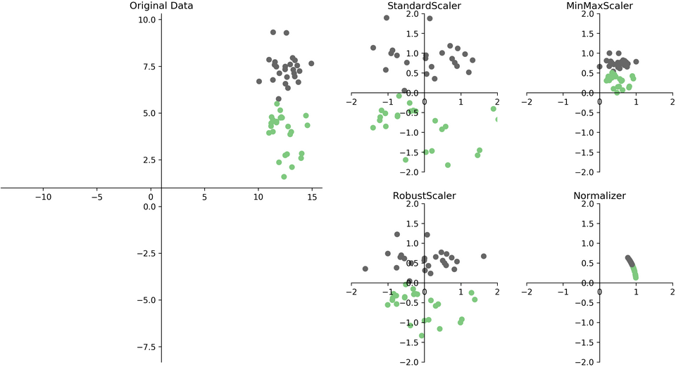 ??? StandardScaler: subtract mean, divide by standard deviation. MinMaxScaler: subtract minimum, divide by range. Afterwards between 0 and 1. Robust Scaler: uses median and quantiles, therefore robust to outliers. Similar to StandardScaler. Normalizer: only considers angle, not length. Helpful for histograms, not that often used. StandardScaler is usually good, but doesn’t guarantee particular min and max values --- class: spacious # Sparse Data - Data with many zeros – only store non-zero entries. - Subtracting anything will make the data “dense” (no more zeros) and blow the RAM. - Only scale, don’t center (use MaxAbsScaler) ??? You have to be careful if you have sparse data. Sparse data is data where most entries of the data-matrix X are zero – often only 1% or less are not zero. You can store this efficiently by only storing the nonzero elements. Subtracting the mean results in all features becoming non-zero! So don’t subtract anything, but you can still scale. MaxAbsScaler scales between -1 and 1 by dividing with the maximum absolute value for each feature. --- # Standard Scaler Example ```python from sklearn.linear_model import Ridge X, y = boston.data, boston.target X_train, X_test, y_train, y_test = train_test_split( X, y, random_state=0) scaler = StandardScaler() scaler.fit(X_train) X_train_scaled = scaler.transform(X_train) ridge = Ridge().fit(X_train_scaled, y_train) X_test_scaled = scaler.transform(X_test) ridge.score(X_test_scaled, y_test) ``` ``` 0.634 ``` ??? Here’s how you do the scaling with StandardScaler in scikit-learn. Similar interface to models, but “transform” instead of “predict”. “transform” is always used when you want a new representation of the data. Fit on training set, transform training set, fit ridge on scaled data, transform test data, score scaled test data. The fit computes mean and standard deviation on the training set, transform subtracts the mean and the standard deviation. We fit on the training set and apply transform on both the training and the test set. That means the training set mean gets subtracted from the test set, not the test-set mean. That’s quite important. --- class: center, middle .center[ 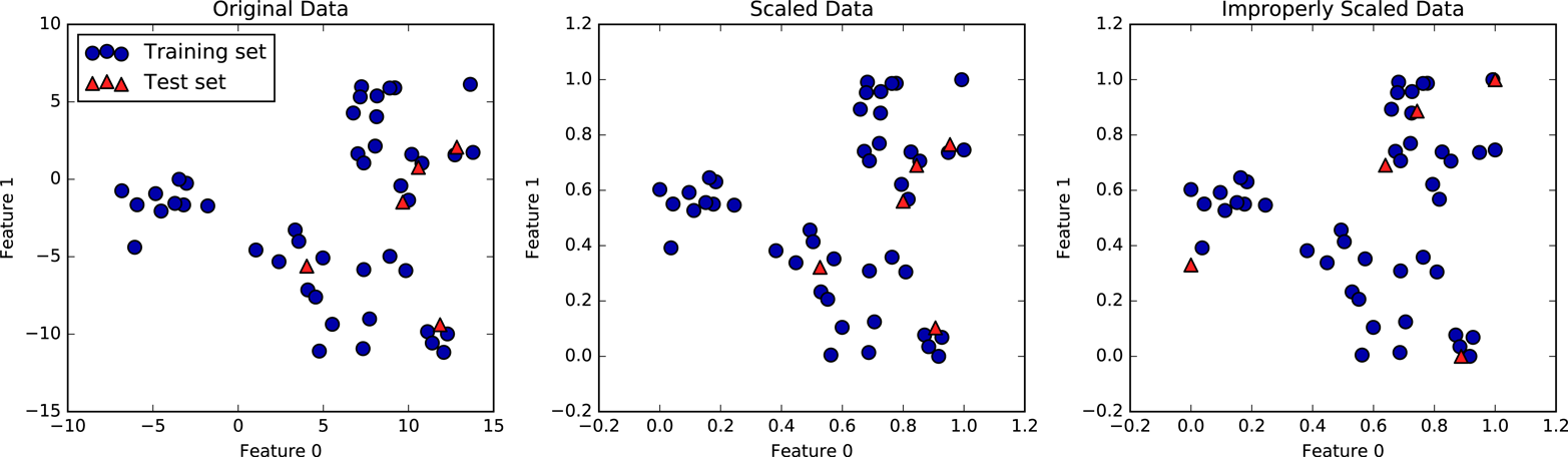 ] ??? Here’s an illustration why this is important using the min-max scaler. Left is the original data. Center is what happens when we fit on the training set and then transform the training and test set using this transformer. The data looks exactly the same, but the ticks changed. Now the data has a minimum of zero and a maximum of one on the training set. That’s not true for the test set, though. No particular range is ensured for the test-set. It could even be outside of 0 and 1. But the transformation is consistent with the transformation on the training set, so the data looks the same. On the right you see what happens when you use the test-set minimum and maximum for scaling the test set. That’s what would happen if you’d fit again on the test set. Now the test set also has minimum at 0 and maximum at 1, but the data is totally distorted from what it was before. So don’t do that. --- class: center, middle # Sckit-Learn API Summary 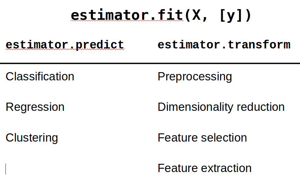 ??? Here’s a summary of the scikit-learn methods. All models have a fit method which takes the training data X_train. If the model is supervised, such as our classification and regression models, they also take a y_train parameter. The scalers don’t use a y_train because they don’t use the labels at all – you could say they are unsupervised methods, but arguably they are not really learning methods at all. Models (also known as estimators in scikit-learn) to make a prediction of a target variable, you use the predict method, as in classification and regression. If you want to create a new representation of the data, a new kind of X, then you use the transform method, as we did with scaling. The transform method is also used for preprocessing, feature extraction and feature selection, which we’ll see later. All of these change X into some new form. There’s two important shortcuts. To fit an estimator and immediately transform the training data, you can use fit_transform. That’s often more efficient then using first fit and then transform. The same goes for fit_predict. --- class: smaller, compact ```python from sklearn.linear_model import Ridge ridge = Ridge() ridge.fit(X_train, y_train) ridge.score(X_test, y_test) ``` ``` 0.717 ``` ```python ridge.fit(X_train_scaled, y_train) ridge.score(X_test_scaled, y_test) ``` ``` 0.718 ``` ```python from sklearn.neighbors import KNeighborsRegressor knn = KNeighborsRegressor() knn.fit(X_train, y_train) knn.score(X_test, y_test) ``` ``` 0.499 ``` ```python knn = KNeighborsRegressor() knn.fit(X_train_scaled, y_train) knn.score(X_test_scaled, y_test) ``` ``` 0.750 ``` ??? Let’s apply the scaler to the Boston housing data. First I used the StandardScaler to scale the training data. Then I applied ten-fold cross-validation to evaluate the Ridge model on the data with and without scaling. I used RidgeCV which automatically picks alpha for me. With and without scaling we get an R^2 of about .72, so no difference. Often there is a difference for Ridge, but not in this case. If we use KneighborsRegressor instead, we see a big difference. Without scaling R^2 is about .5, and with scaling it’s .75. That makes sense since we saw that for distance calculations basically all features are dominated by the TAX feature. However, there is a bit of a problem with the analysis we did here. Can you see it? # Feature Distributions ??? Now that we discussed scaling and pipelines, let’s talk about some more preprocessing methods. One important aspect is dealing with different input distributions. --- class: left, middle .center[ 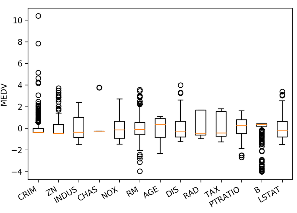 ] ??? Here is a box plot of the boston housing data after transforming it with the standard scaler. Even though the mean and standard deviation are the same for all features, the distributions are quite different. You can see very concentrated distributions like Crim and B, and very skewed distribuations like RAD and Tax (and also crim and B). Many models, in particular linear models and neural networks, work better if the features are approximately normal distributed. Let’s also check out the histograms of the data to see a bit better what’s going on. --- class: left, middle .center[  ] ??? Clearly CRIM and ZN and B are very peaked, and LSTAT and DIS and Age are very asymmetric. Sometimes you can use a hack like applying a logarithm to the data to get better behaved values. There is slightly more rigorous technique though. --- # Power Transformations (Box-Cox & Yeo-Johnson) .left-column[ $$bc_{\lambda}(x) = \cases{\frac{x^\lambda - 1}{\lambda} & \text{if } \lambda \neq 0\cr log(x) & \text{if } \lambda = 0 }$$ ] .right-column[  ] .reset-column[ ```python from sklearn.preprocessing import PowerTransformer # Use "yeo-johnson" for positive+negative data pt = PowerTransformer(method='box-cox') pt.fit(X) ``` ] ??? The Box-Cox transformation is a family of univariate functions to transform your data, parametrized by a parameter lambda. For lamda=1 the function is the identity, for lambda = 2 it is square, lambda =0 is log and there is many other functions in between. For a given dataset, a separate parameter lambda is determined for each feature, by minimizing the skewdness of the data (making skewdness close to zero, not close to -inf), so it is more “gaussian”. The skewdness of a function is a measure of the asymmetry of a function and is 0 for functions that are symmetric around their mean. Unfortunately the Box-Cox transformation is only applicable to positive features. --- .wide-left-column[  ] .narrow-right-column[Before] .clear-column[] .wide-left-column[] .narrow-right-column[After] ??? Here are the histograms of the original data and the transformed data. The title of each subplot shows the estimated lambda. If the lambda is close to 1, the transformation didn’t change much. If it is away from 1, there was a significant transformation. You can clearly see the effect on “CRIM” which was approximately log-transformed, and lstat and nox which were approximately transformed by sqrt. For the binary CHAS the transformation doesn’t make a lot of sense, though. --- .wide-left-column[  ] .narrow-right-column[Before] .clear-column[] .wide-left-column[] .narrow-right-column[After] ??? Here is a comparison of the feature vs response plot before and after the box-cox transformation. The dis, lstat and crim relationships now look a bit more obvious and linear. --- class: left, middle # Discrete features --- class: center, middle # Categorical Variables .larger[ $$ \lbrace 'red', 'green', 'blue' \rbrace \subset ℝ^p ? $$ ] ??? Before we can apply a machine learning algorithm, we first need to think about how we represent our data. Earlier, I said x \in R^n. That’s not how you usually get data. Often data has units, possibly different units for different sensors, it has a mixture of continuous values and discrete values, and different measurements might be on totally different scales. First, let me explain how to deal with discrete input variables, also known as categorical features. They come up in nearly all applications. Let’s say you have three possible values for a given measurement, whether you used setup1 setup2 or setup3. You could try to encode these into a single real number, say 0, 1 and 2, or e, \pi, \tau. However, that would be a bad idea for algorithms like linear regression --- class: center, middle # Categorical Variables .center[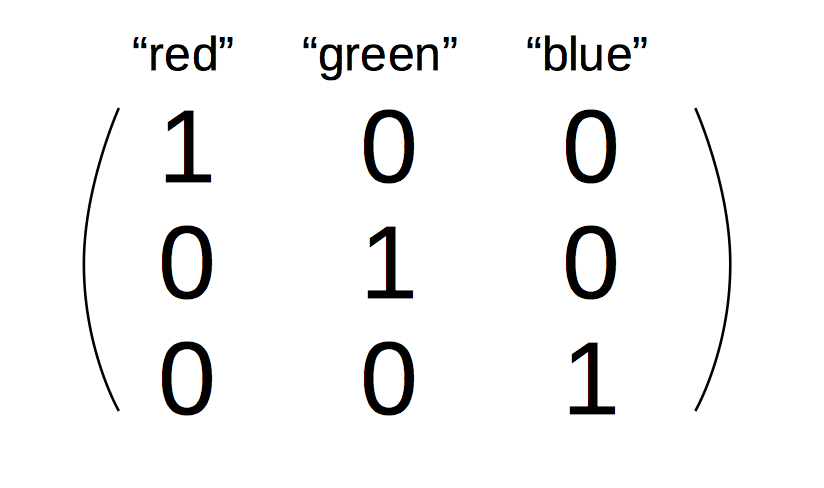] ??? If you encode all three values using the same feature, then you are imposing a linear relation between them, and in particular you define an order between the categories. Usually, there is no semantic ordering of the categories, and so we shouldn’t introduce one in our representation of the data. Instead, we add one new feature for each category, And that feature encodes whether a sample belongs to this category or not. That’s called a one-hot encoding, because only one of the three features in this example is active at a time. You could actually get away with n-1 features, but in machine learning that usually doesn’t matter --- class: center, middle .center[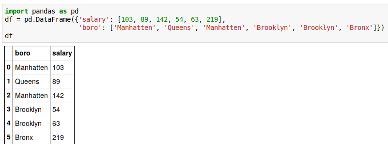] .center[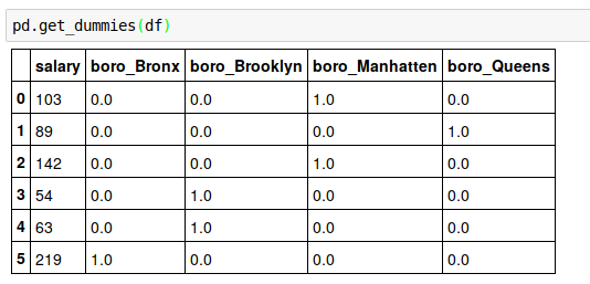] ??? N/A --- class: center, middle .center[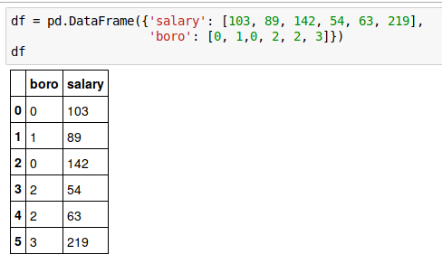] .left-column[] .right-column[] ??? N/A --- class: center, middle .center[] ??? N/A --- class: smaller #Pandas Categorical Columns ```python import pandas as pd df = pd.DataFrame({'salary': [103, 89, 142, 54, 63, 219], 'boro': ['Manhattan', 'Queens', 'Manhattan', 'Brooklyn', 'Brooklyn', 'Bronx']}) df['boro'] = pd.Categorical( df.boro, categories=['Manhattan', 'Queens', 'Brooklyn', 'Bronx', 'Staten Island']) pd.get_dummies(df) ``` ``` salary boro_Manhattan boro_Queens boro_Brooklyn boro_Bronx boro_Staten Island 0 103 1 0 0 0 0 1 89 0 1 0 0 0 2 142 1 0 0 0 0 3 54 0 0 1 0 0 4 63 0 0 1 0 0 5 219 0 0 0 1 0 ``` ??? N/A --- #OneHotEncoder ```python from sklearn.preprocessing import OneHotEncoder df = pd.DataFrame({'salary': [103, 89, 142, 54, 63, 219], 'boro': [0, 1, 0, 2, 2, 3]}) ohe = OneHotEncoder(categorical_features=[0]).fit(df) ohe.transform(df).toarray() ``` ``` array([[ 1., 0., 0., 0., 103.], [ 0., 1., 0., 0., 89.], [ 1., 0., 0., 0., 142.], [ 0., 0., 1., 0., 54.], [ 0., 0., 1., 0., 63.], [ 0., 0., 0., 1., 219.]]) ``` - Legacy mode: Only works for integers right now, not strings. - New mode: works on strings and integers, but always transforms all columns. ??? N/A - Fit-transform paradigm ensures train and test-set categories correspond. --- # OneHotEncoder ```python import pandas as pd df = pd.DataFrame({'salary': [103, 89, 142, 54, 63, 219], 'boro': ['Manhattan', 'Queens', 'Manhattan', 'Brooklyn', 'Brooklyn', 'Bronx']}) ce = OneHotEncoder().fit(df) ce.transform(df).toarray() ``` ``` array([[ 0., 0., 1., 0., 0., 0., 0., 1., 0., 0.], [ 0., 0., 0., 1., 0., 0., 1., 0., 0., 0.], [ 0., 0., 1., 0., 0., 0., 0., 0., 1., 0.], [ 0., 1., 0., 0., 1., 0., 0., 0., 0., 0.], [ 0., 1., 0., 0., 0., 1., 0., 0., 0., 0.], [ 1., 0., 0., 0., 0., 0., 0., 0., 0., 1.]]) ``` - Always transforms all columns ??? - Fit-transform paradigm ensures train and test-set categories correspond. --- # New in 0.20.0 ## OneHotEncoder + ColumnTransformer ```python categorical = df.dtypes == object preprocess = make_column_transformer( (~categorical, StandardScaler()), (categorical, OneHotEncoder()) ``` --- class: some-space #OneHot vs Statisticians - One-hot is redundant (last one is 1 – sum of others) - Can introduce co-linearity - Can drop one - Choice which one matters for penalized models - Keeping all can make the model more interpretable ??? N/A --- class: some-space #Models Supporting Discrete Features - In principle: - All tree-based models, naive Bayes - In scikit-learn: - None - In scikit-learn "soon": - Decision trees, random forests, gradient boosting ??? N/A --- class: center, middle # Dealing with missing values --- class: spacious # Dealing with missing values - Missing values can be encoded in many ways - Numpy has no standard format for it (often np.NaN) - pandas does - Sometimes: 999, ???, ?, np.inf, “N/A”, “Unknown“ … - Not discussing “missing output” - that’s semi-supervised learning. - Often missingness is informative! ??? - Add feature that encodes that data was missing! --- .center[  ] ??? - Problem : Prediction not for all samples ! - Accuracy might be biased --- .center[  ] ??? --- class: spacious # Imputation Methods - Mean / Median - kNN - Regression models - Probabilistic models ??? --- # Mean and Median .center[  ] ??? --- .center[  ] ??? --- class: spacious # KNN Imputation - Find k nearest neighbors that have non-missing values. - Fill in all missing values using the average of the neighbors. - PR in scikit-learn: https://github.com/scikit-learn/scikit-learn/pull/9212 ??? --- .center[  ] --- class: center, middle # Notebook: Preprocessing