class: center, middle  ### Intermediate Machine learning with scikit-learn # Cross Validation and Grid Search Andreas C. Müller Columbia University, scikit-learn .smaller[https://github.com/amueller/ml-workshop-2-of-4] --- class: center # Influence of Number of Neighbors 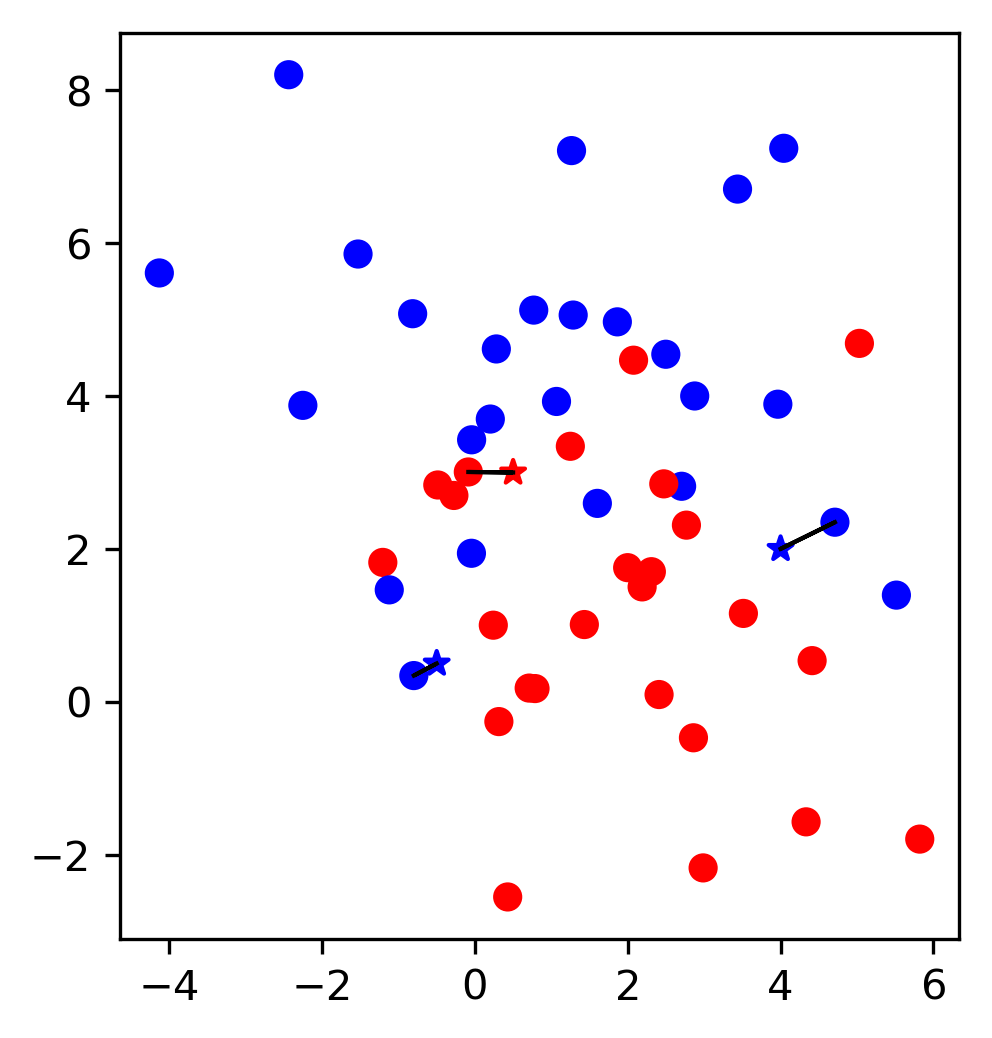 ??? So this was the predictions as made by one-nearest neighbor. But we can also consider more neighbors, for example three. Here is the three nearest neighbors for each of the points and the corresponding labels. We can then make a prediction by considering the majority among these three neighbors. And as you can see, in this case all the points changed their labels! (I was actually quite surprised when I saw that, I just picked some points at random). Clearly the number of neighbors that we consider matters a lot. But what is the right number? The is a problem you’ll encounter a lot in machine learning, the problem of tuning parameters of the model, also called hyper-parameters, which can not be learned directly from the data. --- class: center # Influence of Number of Neighbors 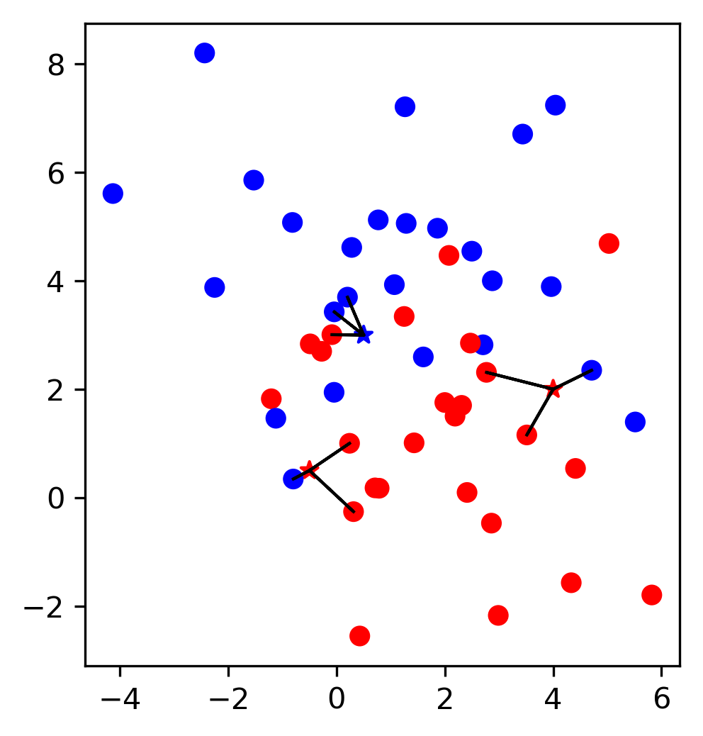 ??? So this was the predictions as made by one-nearest neighbor. But we can also consider more neighbors, for example three. Here is the three nearest neighbors for each of the points and the corresponding labels. We can then make a prediction by considering the majority among these three neighbors. And as you can see, in this case all the points changed their labels! (I was actually quite surprised when I saw that, I just picked some points at random). Clearly the number of neighbors that we consider matters a lot. But what is the right number? The is a problem you’ll encounter a lot in machine learning, the problem of tuning parameters of the model, also called hyper-parameters, which can not be learned directly from the data. --- class: center, some-space # Influence of n_neighbors 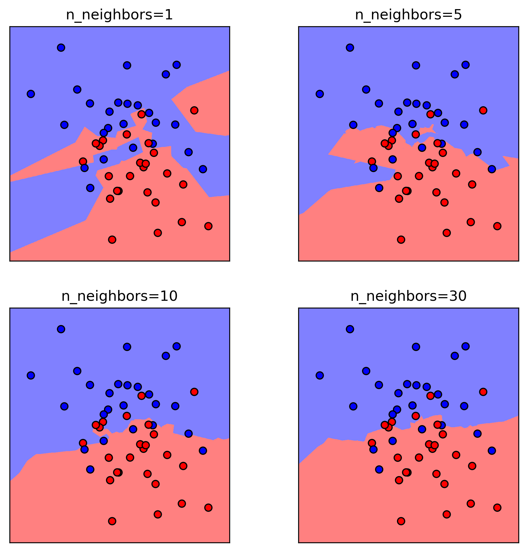 ??? Here’s an overview of how the classification changes if we consider different numbers of neighbors. You can see as red and blue circles the training data. And the background is colored according to which class a datapoint would be assigned to for each location. For one neighbor, you can see that each point in the training set has a little area around it that would be classified according to it’s label. This means all the training points would be classified correctly, but it leads to a very complex shape of the decision boundary. If we increase the number of neighbors, the boundary between red and blue simplifies, and with 40 neighbors we mostly end up with a line. This also means that now many of the training data points would be labeled incorrectly. --- class: center, spacious # Model complexity 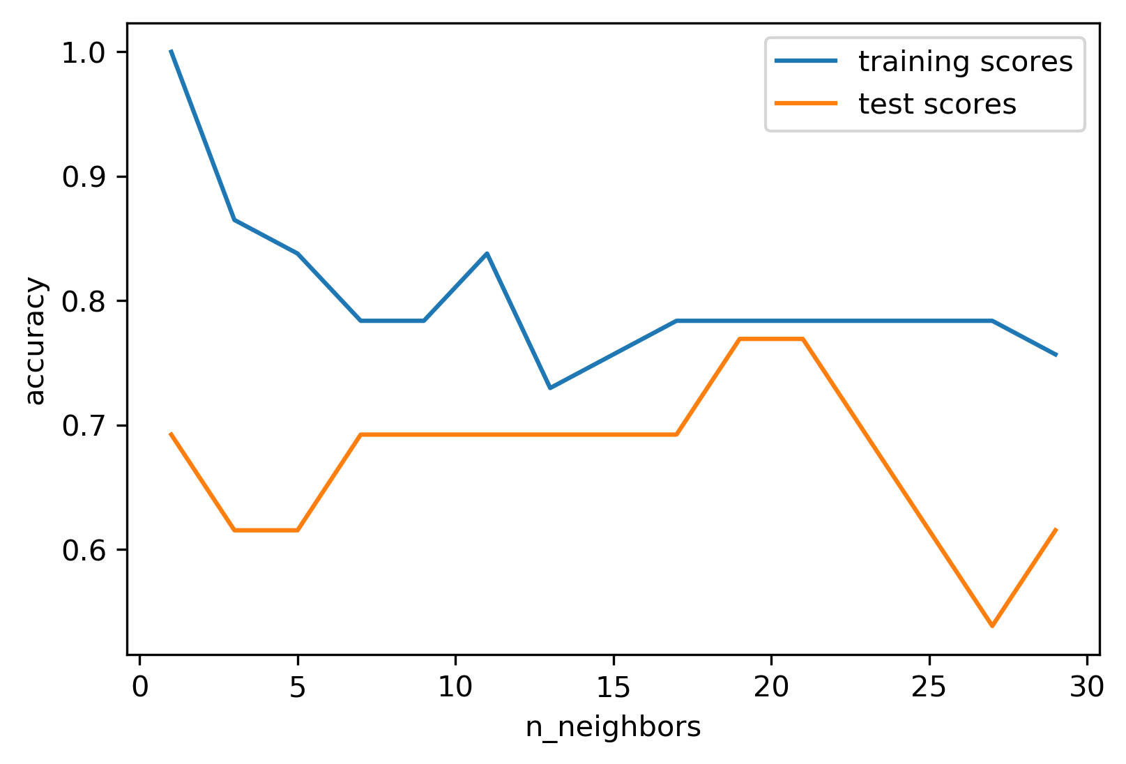 ??? We can look at this in more detail by comparing training and test set scores for the different numbers of neighbors. Here, I did a random 75%/25% split again. This is a very noisy plot as the dataset is very small and I only did a random split, but you can see a trend here. You can see that for a single neighbor, the training score is 1 so perfect accuracy, but the test score is only 70%. If we increase the number of neighbors we consider, the training score goes down, but the test score goes up, with an optimum at 19 and 21, but then both go down again. This is a very typical behavior, that I sketched in a schematic for you. --- class: center, spacious # Overfitting and Underfitting  ??? here is a cartoon version of how this chart looks in general, though it's horizontally flipped to the one with saw for knn. This chart has accuracy on the y axis, and the abstract concept of model complexity on the x axis. If we make our machine learning models more complex, we will get better training set accuracy, as the model will be able to capture more of the variations in the data. --- class: center, spacious # Overfitting and Underfitting  ??? But if we look at the generalization performance, we get a different story. If the model complexity is too low, the model will not be able to capture the main trends, and a more complex model means better generalization. However, if we make the model too complex, generalization performance drops again, because we basically learn to memorize the dataset. --- class: center, spacious # Overfitting and Underfitting  ??? If we use too simple a model, this is often called underfitting, while if we use to complex a model, this is called overfitting. And somewhere in the middle is a sweet spot. Most models have some way to tune model complexity, and we’ll see many of them in the next couple of weeks. So going back to nearest neighbors, what parameters correspond to high model complexity and what to low model complexity? high n_neighbors = low complexity! --- # So far: Train-test-split  ??? So far we’ve work with a split of the data into a training and a test set, build the model on the training set, and evaluated on the test set. So now, lets say we want to adjust the parameter n_neigbhbors in k neighbors algorithm, how could we do this? [split, try out different values of k, choose the best on test set] What’s the problem with that? - good for choosing k, overly optimistic for getting accuracy! --- # Threefold split  ??? The simplest way to combat this overfitting to the test set is by using a three-fold split of the data, into a training, a validation and a test set as we just did. We use the training set for model building, the validation set for parameter selection and the test set for a final evaluation of the model. So how many models should you try out on the test set? Only one! Ideally use use the test-set exactly once, otherwise you make a multiple hypothesis testing error! What are downsides of this? We lose a lot of data for evaluation, and the results depend on the particular sampling. --- class: center # Overfitting the validation set  --- class: center # Overfitting the validation set  --- class: center # Overfitting the validation set  --- class: center # Overfitting the validation set  --- # Threefold Split for Hyper-Parameters .smaller[ ```python X_trainval, X_test, y_trainval, y_test = train_test_split(X, y) X_train, X_val, y_train, y_val = train_test_split(X_trainval, y_trainval) val_scores = [] neighbors = np.arange(1, 15, 2) for i in neighbors: knn = KNeighborsClassifier(n_neighbors=i) knn.fit(X_train, y_train) val_scores.append(knn.score(X_val, y_val)) print(f"best validation score: {np.max(val_scores):.3}") best_n_neighbors = neighbors[np.argmax(val_scores)] print("best n_neighbors:", best_n_neighbors) knn = KNeighborsClassifier(n_neighbors=best_n_neighbors) knn.fit(X_trainval, y_trainval) print(f"test-set score: {knn.score(X_test, y_test):.3f}") ``` ``` best validation score: 0.991 best n_neighbors: 11 test-set score: 0.951 ``` ] ??? FIXME complex code Here is an implementation of the three-fold split for selecting the number of neighbors. For each number of neighbors that we want to try, we build a model on the training set, and evaluate it on the validation set. We then pick the best validation set score, here that’s 97.2%, achieved when using three neighbors. We then retrain the model with this parameter, and evaluate on the test set. The retraining step is somewhat optional. We could also just use the best model. But retraining allows us to make better use of all the data. Still, depending on the test-set size we might be using only 70% or 80% of the data, and our results depend on how exactly we split the datasets. So how can we make this more robust? --- # Cross-validation .center[  ] ??? The answer is of course cross-validation. In cross-validation, you split your data into multiple folds, usually 5 or 10, and built multiple models. You start by using fold1 as the test data, and the remaining ones as the training data. You build your model on the training data, and evaluate it on the test fold. For each of the splits of the data, you get a model evaluation and a score. In the end, you can aggregate the scores, for example by taking the mean. What are the pros and cons of this? Each data point is in the test-set exactly once! Takes 5 or 10 times longer! Better data use (larger training sets). Does that solve all problems? No, it replaces only one of the splits, usually the inner one! -- .smaller[ pro: more stable, more data con: slower ] ??? --- class: center, some-space # Cross-validation + test set  ??? Here is how the workflow looks like when we are using five-fold cross-validation together with a test-set split for adjusting parameters. We start out by splitting of the test data, and then we perform cross-validation on the training set. Once we found the right setting of the parameters, we retrain on the whole training set and evaluate on the test set. --- # Grid-Search with Cross-Validation .smaller[ ```python from sklearn.model_selection import cross_val_score X_train, X_test, y_train, y_test = train_test_split(X, y) cross_val_scores = [] for i in neighbors: knn = KNeighborsClassifier(n_neighbors=i) scores = cross_val_score(knn, X_train, y_train, cv=10) cross_val_scores.append(np.mean(scores)) print(f"best cross-validation score: {np.max(cross_val_scores):.3}") best_n_neighbors = neighbors[np.argmax(cross_val_scores)] print(f"best n_neighbors: {best_n_neighbors}") knn = KNeighborsClassifier(n_neighbors=best_n_neighbors) knn.fit(X_train, y_train) print(f"test-set score: {knn.score(X_test, y_test):.3f}") ``` ``` best cross-validation score: 0.967 best n_neighbors: 9 test-set score: 0.965 ``` ] ??? Here is an implementation of this for k nearest neighbors. We split the data, then we iterate over all parameters and for each of them we do cross-validation. We had seven different values of n_neighbors, and we are running 10 fold cross-validation. How many models to we train in total? 10 * 7 + 1 = 71 (the one is the final model) --- class: center, middle  ??? Here is a conceptual overview of this way of tuning parameters, we start of with the dataset and a candidate set of parameters we want to try, labeled parameter grid, for example the number of neighbors. We split the dataset in to training and test set. We use cross-validation and the parameter grid to find the best parameters. We use the best parameters and the training set to build a model with the best parameters, and finally evaluate it on the test set. Because this is such a common pattern, there is a helper class for this in scikit-learn, called GridSearch CV, which does most of these steps for you. --- # GridSearchCV .smaller[ ```python from sklearn.model_selection import GridSearchCV X_train, X_test, y_train, y_test = train_test_split(X, y, stratify=y) param_grid = {'n_neighbors': np.arange(1, 30, 2)} grid = GridSearchCV(KNeighborsClassifier(), param_grid=param_grid, cv=10, return_train_score=True) grid.fit(X_train, y_train) print(f"best mean cross-validation score: {grid.best_score_}") print(f"best parameters: {grid.best_params_}") print(f"test-set score: {grid.score(X_test, y_test):.3f}") ``` ``` best mean cross-validation score: 0.967 best parameters: {'n_neighbors': 9} test-set score: 0.993 ``` ] ??? Here is an example. We still need to split our data into training and test set. We declare the parameters we want to search over as a dictionary. In this example the parameter is just n_neighbors and the values we want to try out are a range. The keys of the dictionary are the parameter names and the values are the parameter settings we want to try. If you specify multiple parameters, all possible combinations are tried. This is where the name grid-search comes from - it’s an exhaustive search over all possible parameter combinations that you specify. GridSearchCV is a class, and it behaves just like any other model in scikit-learn, with a fit, predict and score method. It’s what we call a meta-estimator, since you give it one estimator, here the KneighborsClassifier, and from that GridSearchCV constructs a new estimator that does the parameter search for you. You also specify the parameters you want to search, and the cross-validation strategy. Then GridSearchCV does all the other things we talked about, it does the cross-validation and parameter selection, and retrains a model with the best parameter settings that were found. We can check out the best cross-validation score and the best parameter setting with the best_score_ and best_params_ attributes. And finally we can compute the accuracy on the test set, simply but using the score method! That will use the retrained model under the hood. --- class: compact # GridSearchCV Results .tiny[ ```python import pandas as pd results = pd.DataFrame(grid.cv_results_) results.columns ``` ``` Index(['mean_fit_time', 'mean_score_time', 'mean_test_score', 'mean_train_score', 'param_n_neighbors', 'params', 'rank_test_score', 'split0_test_score', 'split0_train_score', 'split1_test_score', 'split1_train_score', 'split2_test_score', 'split2_train_score', 'split3_test_score', 'split3_train_score', 'split4_test_score', 'split4_train_score', 'split5_test_score', 'split5_train_score', 'split6_test_score', 'split6_train_score', 'split7_test_score', 'split7_train_score', 'split8_test_score', 'split8_train_score', 'split9_test_score', 'split9_train_score', 'std_fit_time', 'std_score_time', 'std_test_score', 'std_train_score'], dtype='object') ``` ```python results.params ``` ``` 0 {'n_neighbors': 1} 1 {'n_neighbors': 3} 2 {'n_neighbors': 5} 3 {'n_neighbors': 7} 4 {'n_neighbors': 9} 5 {'n_neighbors': 11} 6 {'n_neighbors': 13} Name: params, dtype: object ``` ] ??? FIXME text size GridSearchCV also computes a lot of interesting statistics for you, which are stored in the cv_results_ attribute. That attribute is a dictionary, but it’s easiest to convert it to a pandas dataframe to look at it. Here you can see the columns. Theres mean fit time, mean score time, mean test scores, mean training scores, standard deviations and scores for each individual split of the data. And there is one row for each setting of the parameters we tried out. --- class: center # n_neighbors Search Results  ??? We can use this for example to plot the results of cross-validation over the different parameters. Here are the mean training score and mean test score together with one standard deviation. --- class: spacious # Nested Cross-Validation - Replace outer split by CV loop - Doesn’t yield single model (inner loop might have different best parameter settings) - Takes a long time, not that useful in practice ??? We could additionally replace the outer split of the data by cross-validation. That would yield what’s known as nested cross-validation. This is sometimes interesting when comparing different models, but it will not actually yield one final model. It will yield one model for each loop of the outer fold, which might have different settings of the parameters. Also, this takes a really long time to train, by an additional factor of 5 or 10, so this is not used very commonly in practice. But let’s dive into the cross-validation a bit more. --- class: center, middle # Cross-Validation Strategies ??? So I mentioned k-fold cross validation, where k is usually 5 or ten, but there are many other strategies. One of the most commonly ones is stratified k-fold cross-validation. --- .center[  ] --- class: compact .center[  ] .smallest[ Stratified: Ensure relative class frequencies in each fold reflect relative class frequencies on the whole dataset.] ??? The idea behind stratified k-fold cross-validation is that you want the test set to be as representative of the dataset as possible. StratifiedKFold preserves the class frequencies in each fold to be the same as of the overall dataset. Here is and example of a dataset with three classes that are ordered. If you apply standard three-fold to this, the first third of the data would be in the first fold, the second in the second fold and the third in the third fold. Because this data is sorted, that would be particularly bad. If you use stratified cross-validation it would make sure that each fold has exactly 1/3 of the data from each class. This is also helpful if your data is very imbalanced. If some of the classes are very rare, it could otherwise happen that a class is not present at all in a particular fold. --- # Importance of Stratification .smaller[ ```python y.value_counts() ``` ``` 0 60 1 40 ``` ```python from sklearn.model_selection import cross_val_score, KFold, StratifiedKFold from sklearn.dummy import DummyClassifier dc = DummyClassifier('most_frequent') skf = StratifiedKFold(n_splits=5, shuffle=True) res = cross_val_score(dc, X, y, cv=skf) np.mean(res), res.std() ``` ``` (0.6, 0.0) ``` ```python kf = KFold(n_splits=5, shuffle=True) res = cross_val_score(dc, X, y, cv=kf) np.mean(res), res.std() ``` ``` (0.6, 0.063) ``` ] --- class: spacious # Repeated KFold and LeaveOneOut - LeaveOneOut : KFold(n_folds=n_samples) <br \> High variance, takes a long time <br \> .tiny[(see [Raschka](https://arxiv.org/pdf/1811.12808.pdf) for a review and [Varoquaux](https://hal.inria.fr/hal-01545002/file/paper.pdf) for empirical evaluation)] - Better: ShuffleSplit (aka Monte Carlo) <br \> Repeatedly sample a test set with replacement - Even Better: RepeatedKFold. <br \> Apply KFold or StratifiedKFold multiple times with shuffled data. ??? If you want even better estimates of the generalization performance, you could try to increase the number of folds, with the extreme of creating one fold per sample. That’s called “LeaveOneOut cross-validation”. However, because the test-set is so small every time, and the training sets all have very large overlap, this method has very high variance. A better way to get a robust estimate is to run 5-fold or 10-fold cross-validation multiple times, while shuffling the dataset. --- class: compact .center[  ] .smaller[Number of iterations and test set size independent] ??? Another interesting variant is shuffle split and stratified shuffle split. In shuffle split, we repeatedly sample disjoint training and test sets randomly. You only have to specify the number of iterations, the training set size and the test set size. This also allows you to run many iterations with reasonably large test-sets. It’s also great if you have a very large training set and you want to subsample it to get quicker results. --- class: compact .center[  ] .smaller[ Potentially less variance than StratifiedShuffleSplit.<br /> Five times five fold or at most ten times ten fold is sufficient. ] ??? --- class: spacious # Defaults in scikit-learn - 5-fold in 0.22 (used to be 3 fold) - For classification cross-validation is stratified - train_test_split has stratify option: train_test_split(X, y, stratify=y) - No shuffle by default! ??? By default, all cross-validation strategies are five fold. If you do cross-validation for classification, it will be stratified by default. Because of how the interface is done, that’s not true for train_test_split and if you want a stratified train_test_split, which is always a good idea, you should use stratify=y Another thing that’s important to keep in mind is that by default scikit-learn doesn’t shuffle! So if you run cross-validation twice with the default parameters, it will yield exactly the same results. --- class: center, middle # Cross-Validation with non-iid data ??? --- # Grouped Data ### Assume have data (medical, product, user...) from 5 cities - New York, San Francisco, Los Angeles, Chicago, Houston. We can assume data within a city is more correlated then between cities. ### Usage Scenarios - Assume all future users will be in one of these cities: i.i.d. - Assume we want to generalize to predict for a new city: not i.i.d. ??? Shipped product in 4 cities. Might ship in another one? States: you have all the states, no new state will start to exist Similar thing for multiple measurements per patient. Or geospacial data. ---  ??? A somewhat more complicated approach is group k-fold. This is actually for data that doesn’t fulfill our IID assumption and has correlations between samples. The idea is that there are several groups in the data that each contain highly correlated samples. You could think about patient data where you have multiple samples for each patient, then the groups would be which patient a measurement was taken from. If you want to know how well your model generalizes to new patients, you need to ensure that the measurements from each patient are either all in the training set, or all in the test set. And that’s what GroupKFold does. In this example, there are four groups, and we want three folds. The data is divided such that each group is contained in exactly one fold. There are several other cross-validation methods in scikit-learn that use these groups. --- class: center # Correlations in time (and/or space)  ??? Not necessarily obvious that there is a time component! Data collection usually happens over time! --- class: center # Correlations in time (and/or space)  ??? Not necessarily obvious that there is a time component! Data collection usually happens over time! --- class: center # Correlations in time (and/or space)  ??? Not necessarily obvious that there is a time component! Data collection usually happens over time! ---  ??? Another common case of data that’s not independent is time series. Usually todays stock price is correlated with yesterdays and tomorrows. If you randomly split time series, this makes predictions deceivingly simple. In applications, you usually have data up to some point, and then try to make predictions for the future, in other words, you’re trying to make a forecast. The TimeSeriesSplit in scikit-learn simulates that, by taking increasing chunks of data from the past and making predictions on the next chunk. This is quite different from the other was to do cross-validation, in that the training sets are all overlapping, but it’s more appropriate for time-series. ---  ??? Another common case of data that’s not independent is time series. Usually todays stock price is correlated with yesterdays and tomorrows. If you randomly split time series, this makes predictions deceivingly simple. In applications, you usually have data up to some point, and then try to make predictions for the future, in other words, you’re trying to make a forecast. The TimeSeriesSplit in scikit-learn simulates that, by taking increasing chunks of data from the past and making predictions on the next chunk. This is quite different from the other was to do cross-validation, in that the training sets are all overlapping, but it’s more appropriate for time-series. --- # Using Cross-Validation Generators .tiny[ ```python from sklearn.model_selection import KFold, StratifiedKFold, ShuffleSplit, RepeatedStratifiedKFold kfold = KFold(n_splits=5) skfold = StratifiedKFold(n_splits=5, shuffle=True) ss = ShuffleSplit(n_splits=20, train_size=.4, test_size=.3) rs = RepeatedStratifiedKFold(n_splits=5, n_repeats=10) print("KFold:") print(cross_val_score(KNeighborsClassifier(), X, y, cv=kfold)) print("StratifiedKFold:") print(cross_val_score(KNeighborsClassifier(), X, y, cv=skfold)) print("ShuffleSplit:") print(cross_val_score(KNeighborsClassifier(), X, y, cv=ss)) print("RepeatedStratifiedKFold:") print(cross_val_score(KNeighborsClassifier(), X, y, cv=rs)) ``` ``` KFold: [ 0.93 0.96 0.96 0.98 0.96] StratifiedKFold: [0.98 0.96 0.96 0.97 0.96] ShuffleSplit: [0.98 0.96 0.96 0.98 0.94 0.96 0.95 0.98 0.97 0.92 0.94 0.97 0.95 0.92 0.98 0.98 0.97 0.94 0.97 0.95] RepeatedStratifiedKFold: [0.99 0.96 0.97 0.97 0.95 0.98 0.97 0.98 0.97 0.96 0.97 0.99 0.94 0.96 0.96 0.98 0.97 0.96 0.96 0.97 0.97 0.96 0.96 0.96 0.98 0.96 0.97 0.97 0.97 0.96 0.96 0.95 0.96 0.99 0.98 0.93 0.96 0.98 0.98 0.96 0.96 0.95 0.97 0.97 0.96 0.97 0.97 0.97 0.96 0.96] ``` ] ??? Ok, so how do we use these cross-validation generators? We can simply pass the object to the cv parameter of the cross_val_score function, instead of passing a number. Then that generator will be used. Here are some examples for k-neighbors classifier. We instantiate a Kfold object with the number of splits equal to 5, and then pass it to cross_val_score. We can do the same with StratifiedKFold, and we can also shuffle if we like, or we can use Shuffle split. --- # cross_validate function .smaller[ ```python from sklearn.model_selection import cross_validate res = cross_validate(KNeighborsClassifier(), X, y, return_train_score=True, scoring=["accuracy", "roc_auc"]) res_df = pd.DataFrame(res) ``` ``` fit_time score_time test_accuracy test_roc_auc train_accuracy train_roc_auc 0.000839 0.010204 0.965217 0.996609 0.980176 0.997654 0.000870 0.014424 0.956522 0.983689 0.975771 0.998650 0.000603 0.009298 0.982301 0.999329 0.971491 0.996977 0.000698 0.006670 0.955752 0.984071 0.978070 0.997820 0.000611 0.006559 0.964602 0.994634 0.978070 0.998026 ``` ] ??? FIXME alignment --- class: center, middle # Notebook: Cross-validation and grid search