Linear Models for Regression

class: center, middle

![:scale 40%](images/sklearn_logo.png)

### Intermediate Machine learning with scikit-learn

# Linear Models for Regression

Andreas C. Müller

Columbia University, scikit-learn

.smaller[https://github.com/amueller/ml-workshop-2-of-4]

---
class:center

# Linear Models for Regression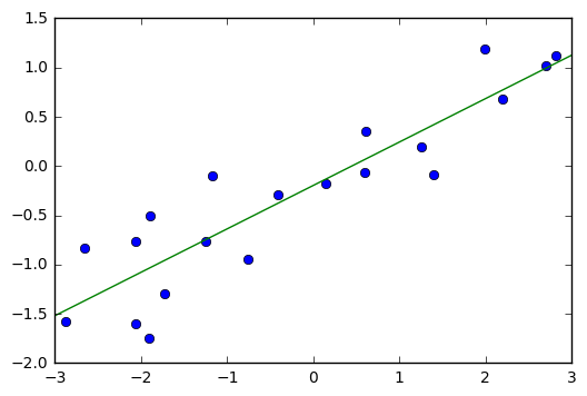

![:scale 50%](images/linear_regression_1d.png)

$$\hat{y} = w^T \mathbf{x} + b = \sum_{i=1}^p w_i x_i +b$$

???
Predictions in all linear models for regression are of the
form shown here: It's an inner product of the features with
some coefficient or weight vector w, and some bias or
intercept b. In other words, the output is a weighted sum of
the inputs, possibly with a shift. here i runs over the
features and x_i is one feature of the data point x. These
models are called linear models because they are linear in
the parameters w. The way I wrote it down here they are also
linear in the features x_i. However, you can replace the
features by any non-linear function of the inputs, and it'll
still be a linear model.

There are many differnt linear models for regression, and
they all share this formula for making predictions. The
difference between them is in how they find w and b based on
the training data.

---
# Ordinary Least Squares

$$\hat{y} = w^T \mathbf{x} + b = \sum_{i=1}^p w_i x_i +b $$

`$$\min_{w \in \mathbb{R}^p, b\in\mathbb{R}} \sum_{i=1}^n (w^T\mathbf{x}_i + b - y_i)^2$$`

Unique solution if $\mathbf{X} = (\mathbf{x}_1, ... \mathbf{x}_n)^T$ has full column rank.
???
The most straight-forward solution that goes back to Gauss
is ordinary least squares. In ordinary least squares, find w
and b such that the predictions on the training set are as
accurate as possible according the the squared error. That
intuitively makes sense: we want the predictions to be good
on the training set. If there is more samples than features
(and the samples span the whole feature space), then there
is a unique solution. The problem is what's called a least
squares problem, which is particularly easy to optimize and
get the unique solution to.

However, if there are more features than samples, there are
usually many perfect solutions that lead to 0 error on the
training set. Then it's not clear which solution to pick.
Even if there are more samples than features, if there are
strong correlations among features the results might be
unstable, and we'll see some examples of that soon.

Before we look at examples, I want to introduce a popular
alternative.

---
# Ridge Regression

`$$ \min_{w \in \mathbb{R}^p, b\in\mathbb{R}} \sum_{i=1}^n (w^T\mathbf{x}_i + b - y_i)^2 + \alpha ||w||^2 $$`

Always has a unique solution.

Tuning parameter alpha.

???
In Ridge regression we add another term to the optimization
problem. Not only do we want to fit the training data well,
we also want w to have a small squared l2 norm or squared
euclidean norm. The idea here is that we're decreasing the
"slope" along each of the feature by pushing the
coefficients towards zero. This constraings the model to be
more simple.

So there are two terms in this optimization problem, which
is also called the objective function of the model: the data
fitting term here that wants to be close to the training
data according to the squared norm, and the prenalty or
regularization term here that wants w to have small norm,
and that doesn't depend on the data.

Usually these two goals are somewhat opposing. If we made w
zero, the second term would be zero, but the predictions
would be bad. So we need to trade off between these two. The
trade off is problem specific and is specified by the user.
If we set alpha to zero, we get linear regression, if we set
alpha to infinity we get a constant model. Obviously usually
we want something in between.

This is a very typical example of a general principle in
machine learning, called regularized empirical risk
minimization.

---
# (regularized) Empirical Risk Minimization

`$$ \min_{f \in F} \sum_{i=1}^n L(f(\mathbf{x}_i), y_i) + \alpha R(f) $$`

???
FIXME pointers data fitting / regularization!

Many models in machine learning, like linear models, SVMs
and neural networks follow the general framework of
empirical risk minimization, which you can see here. We
formulate the machine learning problem as an optimization
problem over a family of functions. In our case that was the
family of linear functions parametrized by w and b. The
minimization problem consists of two parts, the data fitting
part and the model complexity part. The data fitting part
says that the predictions mad eby our functions should be
accurate according to some loss L. For our regression
problems that was the squared loss. The model complexity
part says that we prefer simple models and penalizes
complicated f. Most machine learning algorithms can be cast
into this, with a particular choice of family of functions
f, loss function L and regularizer R. And most of machine
learning theory is build around this framework. People proof
for differnt choices of F and L and R that if you minimize
this, you'll be able to generalize well. And that makes
intuitive sense. To do well on the test set, we definitely
want to do reasonably well on the training set. We don't
expect that we can do better on a test set than the training
set. But we also want to minimize the performance difference
between training and test set. If we restrict our model to
be simple via the regularizer R, we have better chances of
the model generalizing.

---
# Reminder on model complexity

![:scale 80%](images/overfitting_underfitting_cartoon_full.png)

???
I hope this sounds familiar from what we talked about last
time. This is a particular way of dealing with overfitting
and underfitting. For this framework in general, or for
ridge regression in particular, trading off the data fitting
and the regularization changes the model complexity. If we
set alpha high we restrict the model, and we will be on the
left side of the graph. If we make alpha small, we allow the
model to fit the data more, and we're on the right side of
the graph.

---
# Ames Housing Dataset

![:scale 80%](images/ames_housing_scatter.png)
.tiny[
```python
print(X.shape)
print(y.shape)
```
```
(2195, 79)
(2195,)
```
]
???
Ok after all this pretty abstract talk, let's make this
concrete. Let's do some regression on the boston housing
dataset. After the last homework you're hopefully familiar
with it. The idea is to predict prices of property in the
boston area in different neighborhoods. This is a dataset
from the 70s I think, so everything is pretty cheap. Most of
the features you can see are continuous, with the exception
of the charlston river variable which says whether the
neighborhood is on the river.

Keep in mind that this data lives in a 13 dimensional space
and these univariate plots only look at 13 different
projections of the data, and can't capture any of the
interactions.

But still we can see that the price clearly depends on some
of these variables. It's also pretty clear that the
dependency is non-linear for some of the variables. We'll
still start with a linear model, because its a very simple
class of models, and I'd always star approaching any model
from the simplest baseline. In this case it's linear
regression. We're having 506 samples and 13 features. We
have much more samples than features. Linear regression
should work just fine. Also it's a tiny dataset, so
basically anything we'll try will run instantaneously, which
is also good to keep in mind.

Another thing that you can see in this graph is that the
features have very different scales. Here's a box plot that
shows that even more clearly.
---

![:scale 100%](images/ames_scaling.png)

???
That's something that will trip up the distance based models
models we talked about last time, as well as the linear
models we're talking about today.  For the penalized models
the different scales mean that different features are
penalized differently, which you usually want to avoid.
Usually there is no particular semantics attached to the
fact that one feature has different magnitutes than another.
We could measure something in inches instead of miles, and
that would change the outcome of the model. That's certainly
not something we want. A good idea is to scale the data to
get rid of this effect. We'll talk about that and other
preprocessing methods in-depth on Wednesday next week. Today
I'm mostly gonna ignore this. But let's get started with
Linear Regression

---
# Coefficient of determination R^2

`$$ R^2(y, \hat{y}) = 1 - \frac{\sum_{i=0}^{n - 1} (y_i - \hat{y}_i)^2}{\sum_{i=0}^{n - 1} (y_i - \bar{y})^2} $$`

`$$ \bar{y} =  \frac{1}{n} \sum_{i=0}^{n - 1} y_i$$`

Can be negative for biased estimators - or the test set!

???
The scores are R squared or coefficient of determination.
This is basically a score that's usually between zero and
one, where one means perfect prediction or perfect
correlation and zero means a random prediction. What it does
is it computes the mean of the targets over the data you're
evaluating it on and then it looks at the distance between
the prediction and the ground truth relative to the mean. If
it's negative, it means you do a worse job at predicting and
just predicting the mean. It can happen if your model was
really bad and bias. The other reason is if you use a test
set. This is guaranteed to be positive on the data it was
fit on with an unbiased linear model, which will nearly
never apply to what we’re doing.

The R^2 can be misleading if there's outliers in the training
data and some consider it a bad metric. Max Kuhn, author of APM
thinks it's a bad metric. It's not clear to me that MSE is much
better in general, though. Reducing anything to a single number
is tricky.

---
class: smaller
# Preprocessing
```python
cat_preprocessing = make_pipeline(
    SimpleImputer(strategy='constant', fill_value='NA'),
    OneHotEncoder(handle_unknown='ignore'))

cont_preprocessing = make_pipeline(
    SimpleImputer(),
    StandardScaler())

preprocess = make_column_transformer(
    (cat_preprocessing, make_column_selector(dtype_include='object')),
    remainder=cont_preprocessing)

X_train, X_test, y_train, y_test = train_test_split(
    X, y, random_state=0)

X_train_pre = preprocess.fit_transform(X_train)
ridge = Ridge().fit(X_train_pre, y_train)

X_test_pre = preprocess.transform(X_test)
ridge.score(X_test_pre)
```
```
0.95
```
???
Let’s look at two simple models. Linear regression and Ridge
regression. What I've done is I’ve split the data into
training and test set and used 10 fold cross-validation to
evaluate them. Here I use cross_val_score together with the
model, the training data, training labels, and 10 fold
cross-validation. This will return 10 scores and I'm going
to compute the mean of them. I'm doing this for both linear
regression and Ridge regression. Here is ridge regression
uses a default value of alpha of 1. Here these two scores
are quite similar.

---

.smallest[
```python
from sklearn.model_selection import GridSearchCV
param_grid = {'alpha': np.logspace(-3, 3, 13)}
print(param_grid)
```
```
{'alpha': array([ 0.001,  0.003, 0.01, 0.032, 0.1, 0.316, 1., 3.162,
                    10., 31.623, 100., 316.228, 1000.])}
```

```python
grid = GridSearchCV(Ridge(), param_grid, cv=10)
grid.fit(X_train, y_train)
```
]
.center[
![:scale 50%](images/ridge_alpha_search.png)
]

???
Coming back to the ridge regression we used the standard
alpha of one which is a reasonable default, but by no means,
this is guaranteed to make sense in this particular problem.
Here I’ve done the grid search. As we talked about on
Monday, I defined a parameter grid where the key is the
parameter I want to search (alpha in Ridge) and the
parameters I want to try. For regularization parameters,
like alpha, it’s usually good to do them on the logarithmic
grid. I do a relatively fine grid here with 13 different
points mostly because I wanted to have a nice plot. In
reality, I would use a three or six or something like that.
I’ve instantiated GridSearchCV with Ridge(), the parameter
grid and do 10 fold cross-validation and then I called
grid.fit. I’ve reported the mean training accuracy and mean
test accuracy over 10 cross-validation folds for each of the
parameter settings. Okay, you can see a couple things here.
A) There's a lot of uncertainty B) The training set is
always better than the test set. C) The most important thing
that you can see here is that regularization didn't help.
Making alpha as small as possible is the best. What I'm
going to do next is I'm going to modify this dataset a
little bit so that we can see the effect of the
regularization. I’m going to modifying by using a polynomial
expansion, again we're going to talk about a little bit more
on Wednesday.

---
.padding-top[
.left-column[
![:scale 100%](images/ridge_alpha_search.png)
]
.right-column[
![:scale 100%](images/ridge_alpha_search_cv_runs.png)
]
]
---
# Triazine Dataset

```python
triazines = fetch_openml('triazines')
triazines.data.shape
```
```
(186, 60)
```
```python
pd.Series(triazines.target).hist()
```
.center[
![:scale 40%](images/triazine_bar.png)
]

---
```python
X_train, X_test, y_train, y_test = train_test_split(
    triazines.data, triazines.target, random_state=0)

cross_val_score(LinearRegression(), X_train, y_train, cv=5)
```
```
array([-4.749e+24, -9.224e+24, -7.317e+23, -2.318e+23, -2.733e+22])
```
```python
cross_val_score(Ridge(), X_train, y_train, cv=5)
```
```
array([0.263, 0.455, 0.024, 0.23 , 0.036])
```

---
```python
param_grid = {'alpha': np.logspace(-3, 3, 13)}

grid = GridSearchCV(Ridge(), param_grid, cv=RepeatedKFold(10, 5),
                    return_train_score=True)
grid.fit(X_train, y_train)
```
.center[
![:scale 40%](images/ridge_alpha_triazine.png)
]

---
# Plotting coefficient values (LR)

```python
lr = LinearRegression().fit(X_train, y_train)
plt.scatter(range(X_train.shape[1]), lr.coef_,
            c=np.sign(lr.coef_), cmap='bwr_r')
```
.center[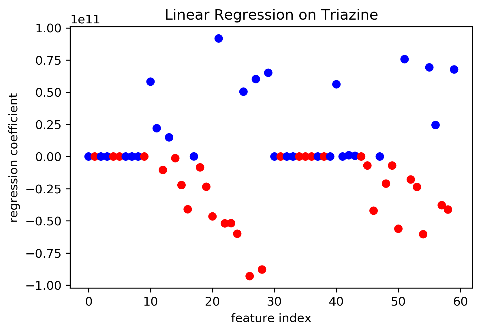
![:scale 55%](images/lr_coefficients_large.png)
]

???
In the previous slide, linear regression did nearly as well
as the Ridge Regression with the default parameters but
let's look at the coefficients of a linear model. These are
the coefficients of the linear model trained on the
polynomial futures. I plot them adding a color to represent
positive and negative. The magnitude here is 1 and then 13
zeros. We have two features, one is like, probably more than
trillions times two and then there's another one that's very
negative. What I conclude from this is, these 2 features are
very highly correlated. The model makes both of them really,
really big and then they cancel each other out. This is not
a very nice model, because it relates to American stability
and also it tells me that these 2 features are like
extremely important, but they might not be important at all.
Like the other features might be more important, but they're
nullified by this cancellation effect. They (0.2 and -0.8)
need to cancel each other out because the predictions are
reasonable and all the houses only cost like $70,000.

---
# Ridge Coefficients

```python
ridge = grid.best_estimator_
plt.scatter(range(X_train.shape[1]), ridge.coef_,
            c=np.sign(ridge.coef_), cmap="bwr_r")
```
.center[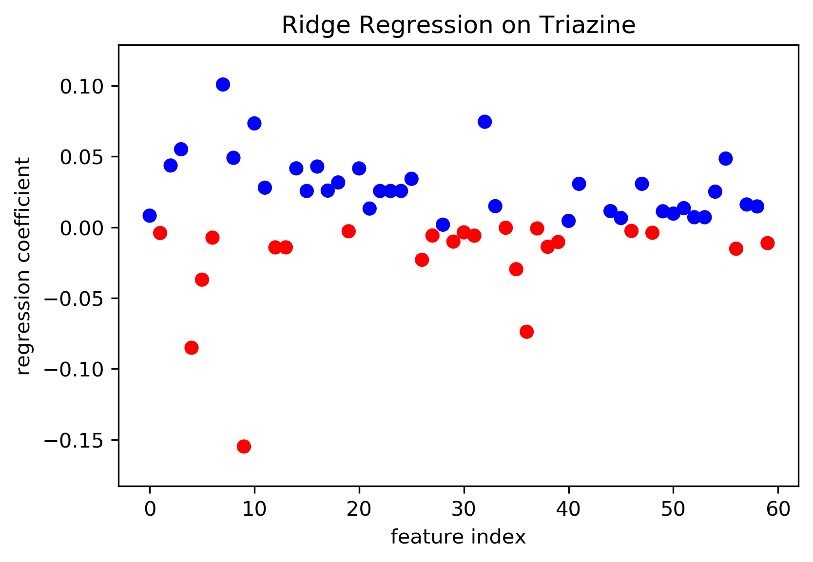
![:scale 55%](images/ridge_coefficients.png)
]

???
Let's look at the Ridge model. This is the best estimator,
which is the model that was found in a grid search with the
best parameter settings. This looks much more reasonable.
This feature, which was a very negative one, still is very
negative. But now this is actually three and minus three. So
this is a much more reasonable range. We can also look at
the features and the effect of different values of alpha.
Here is a Ridge with 3 different values of alpha. In the
previous random seat, alpha equal to 14 was the best now and
now we have it equal to 30 something. The green one is more
or less the best setting and then there's a smaller and a
bigger one. You can see that basically what alpha does is,
on average, it pushes all the coefficients toward zero. So
here you can see this coefficient shrank going from 1 to 14
going to 0 and the same here. So basically, they all push
the different features towards 0. If you look at this long
enough, you can see things that are interesting, the first
one with alpha equal to one it's positive, and with alpha
equal to 100, it's negative. That means depending on how
much you regularize the direction of effect goes in opposite
directions, what that tells me is don't interpret your
models too much because clearly, either it has a positive or
negative effect, it can't have both.

---
```python
ridge100 = Ridge(alpha=100).fit(X_train, y_train)
ridge1 = Ridge(alpha=.1).fit(X_train, y_train)
plt.figure(figsize=(8, 4))

plt.plot(ridge1.coef_, 'o', label="alpha=.1")
plt.plot(ridge.coef_, 'o', label=f"alpha={ridge.alpha:.2f}")
plt.plot(ridge100.coef_, 'o', label="alpha=100")
plt.legend()
```

.center[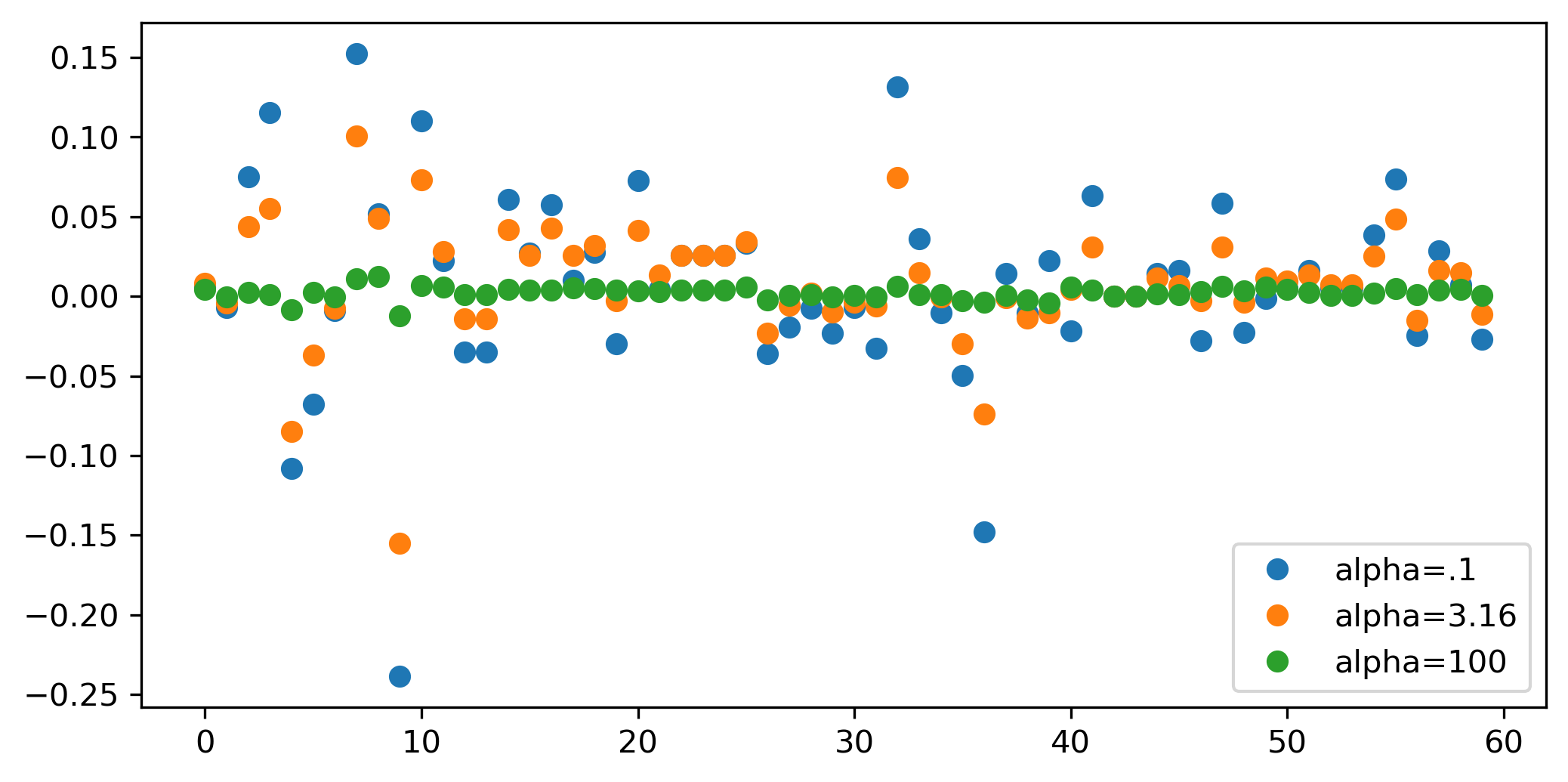
![:scale 60%](images/ridge_coefficients_alpha.png)
]

???

One other way to visualize the coefficient is to look at the
coefficient path or regularization path. On the x-axis is
the alpha, and on the y-axis, the coefficient magnitude.
Basically, I looped over all of the different alphas and you
can see how they shrink towards zero to increase alpha.
There are some very big coefficients that go to zero very
quickly and some coefficients here that stay the same for a
long time.

---
# Lasso Regression

`$$ \min_{w \in \mathbb{R}^p, b\in\mathbb{R}} \sum_{i=1}^n (w^T\mathbf{x}_i + b - y_i)^2 + \alpha ||w||_1 $$`

- Shrinks w towards zero like Ridge

- Sets some w exactly to zero - automatic feature selection!

???
Lasso Regression looks very similar to Ridge Regression. The
only thing that is changed is we use the L1 norm instead of
the L2 norm. L2 norm is the sum of squares, the L1 norm is
the sum of the absolute values. So again, we are shrinking w
towards 0, but we're shrinking it in a different way. The L2
norm penalizes very large coefficients more, the L1 norm
penalizes all coefficients equally. What this does in
practice is its sets some entries of W to exactly 0. It does
automatic feature selection if the coefficient of zero means
it doesn't influence the prediction and so you can just drop
it out of the model. This model does features selection
together with prediction. Ideally what you would want is,
let's say you want a model that does features selections.
The goal is to make our model automatically select the
features that are good. What you would want to penalize the
number of features that it uses, that would be L0 norm.

---
# Grid-Search for Lasso
```python
param_grid = {'alpha': np.logspace(-3, 0, 13)}
print(param_grid)
```
```
{'alpha': array([ 0.001,  0.003, 0.01, 0.032, 0.1, 0.316, 1., 3.162,
                    10., 31.623, 100., 316.228, 1000.])}
```
```python
grid = GridSearchCV(Lasso(normalize=True), param_grid, cv=10)
grid.fit(X_train, y_train)

print(grid.best_params_)
print(grid.best_score_)
```
```
{'alpha': 0.0016}
0.163
```

???

Now we can do Grid Search again, the default parameters
usually don't work very well for Lasso. I use alpha on the
logarithmic grid. I fitted and then I get the best score.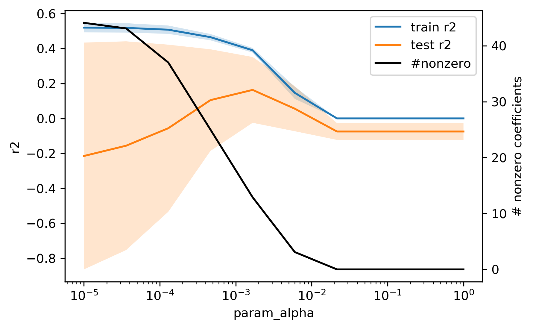
---

![:scale 90%](images/lasso_alpha_triazine.png)

???

Looking at the training test set performance, you can see
that if you increase the regularization, this model gets
really bad. The ridge regression didn't go this badly. If
you set the realization to one, all coefficients become
zero. Other than that there's reasonable performance, which
is about as good as the ridge performance.
---
.center[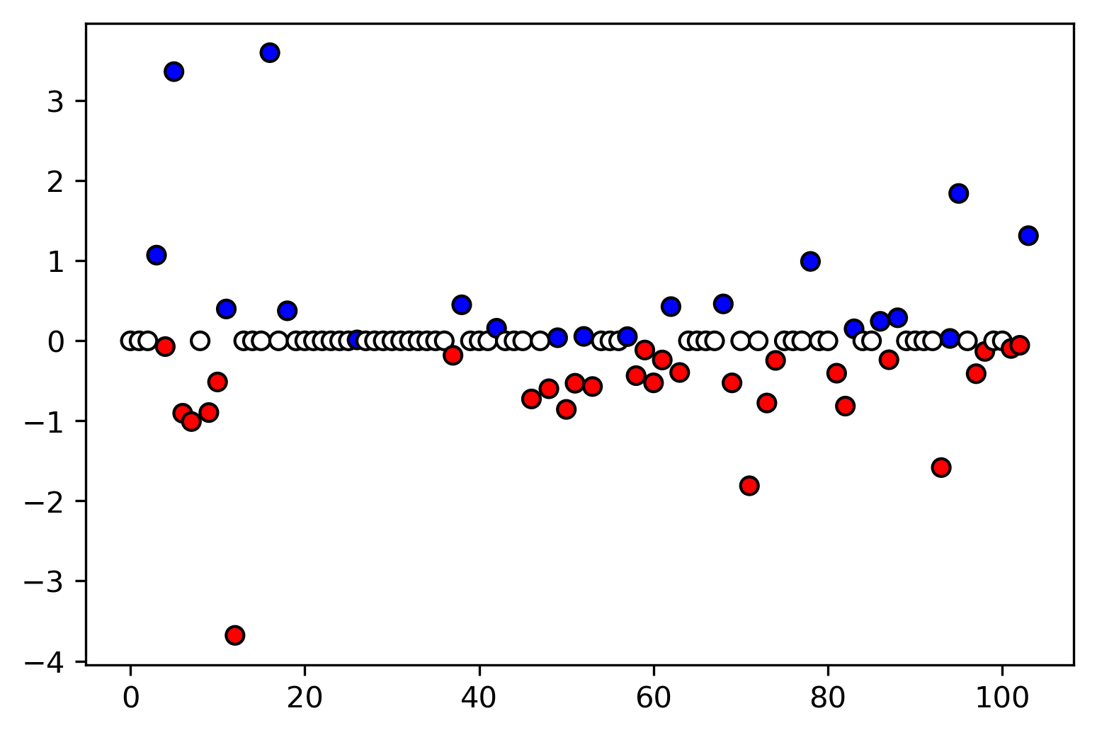
![:scale 60%](images/lasso_coefficients.png)
]

```python
print(X_train.shape)
np.sum(lasso.coef_ != 0)
```
```
(139, 60)
13
```

???

These are the coefficients of the model. Out of the 104
features, it only selected 64 that are non-zero, the other
ones are exactly zero. You can see this visualized here. The
white ones are exactly zero and the other ones on non-zero.
If I wanted I could prune the future space a lot and that
makes the model possibly more interpretable. There's a
slight caveat here if two of the features that are very
correlated, Lasso will pick one of them at random and make
the other one zero. Just because something's zero doesn't
mean it's not important. It means you can drop it out of
this model. If you have two features that are identical, one
of them will be zero and one of them will be not zero and
it's going to be randomly selected. That makes
interpretation a little bit harder.

---
# Elastic Net

- Combines benefits of Ridge and Lasso

- two parameters to tune.

`$$\min_{w \in \mathbb{R}^p, b\in\mathbb{R}} \sum_{i=1}^n ||w^T\mathbf{x}_i + b - y_i||^2 + \alpha_1 ||w||_1 +  \alpha_2 ||w||^2_2 $$`

???
You can also combine them. This actually what works best in
practice. This is what's called the Elastic Net. Elastic Net
tries to combine both of these penalizations together. You
now have both terms, you have the L1 norm and the L2 norm
and you have different values of alpha. Basically, this
generalizes both. If you choose both these are alpha, it can
become ridge and it can become Lasso, it can become any
anything in between. Generally, ridge helps generalization.
So it's a good idea to have the ridge penalty in there, but
also maybe if there are some features that are really not
useful, the L1 penalty helps makes the same exactly zero.

---
# Parametrization in scikit-learn
`$$\min_{w \in \mathbb{R}^p, b\in\mathbb{R}} \sum_{i=1}^n (w^T\mathbf{x}_i + b - y_i)^2 + \alpha \eta ||w||_1 +  \alpha (1 - \eta) ||w||^2_2 $$`

Where $\eta$ is the relative amount of l1 penalty (`l1_ratio` in the code).
???
The way this parameterize in scikit-learn is slightly
different. In scikit-learn, you have a parameter alpha,
which is the amount of regularization and then there's a
parameter called l1_ratio, that says how much of the penalty
should be L1 and L2. If you make this one, you have Lasso,
if you make it zero, you have a Ridge. Don't use Lasso or
Ridge and set alpha zero, because the solver will not handle
it well. If you actually want alpha equal to zero, use
linear regression. Now we have more parameters to tune, but
we just have a more general model. This actually works
pretty well often.

---
# Grid-searching ElasticNet

```python
from sklearn.linear_model import ElasticNet
param_grid = {'alpha': np.logspace(-4, -1, 10),
              'l1_ratio': [0.01, .1, .5, .8, .9, .95, .98, 1]}

grid = GridSearchCV(ElasticNet(), param_grid, cv=10)
grid.fit(X_train, y_train)

print(grid.best_params_)
print(grid.best_score_)
```
```
{'alpha': 0.001, 'l1_ratio': 0.9}
0.100
```
```python
(grid.best_estimator_.coef_!= 0).sum()
```
```
10
```
???
Here is me doing a grid search. If you have two parameters
for the grid search it will do all possible combinations.
Here I do a logarithmic space for alpha and for the
l1_ratio, I use something that’s very close to zero and
something that's very close to one and some stuff in
between. If you want to analyze the output of a 2D grid
search a little bit harder we can’t do the nice curve
anymore.

---
class: smaller
# Analyzing grid-search results
```python
import pandas as pd
res = pd.pivot_table(pd.DataFrame(grid.cv_results_),
    values='mean_test_score', index='param_alpha', columns='param_l1_ratio')
```
.center[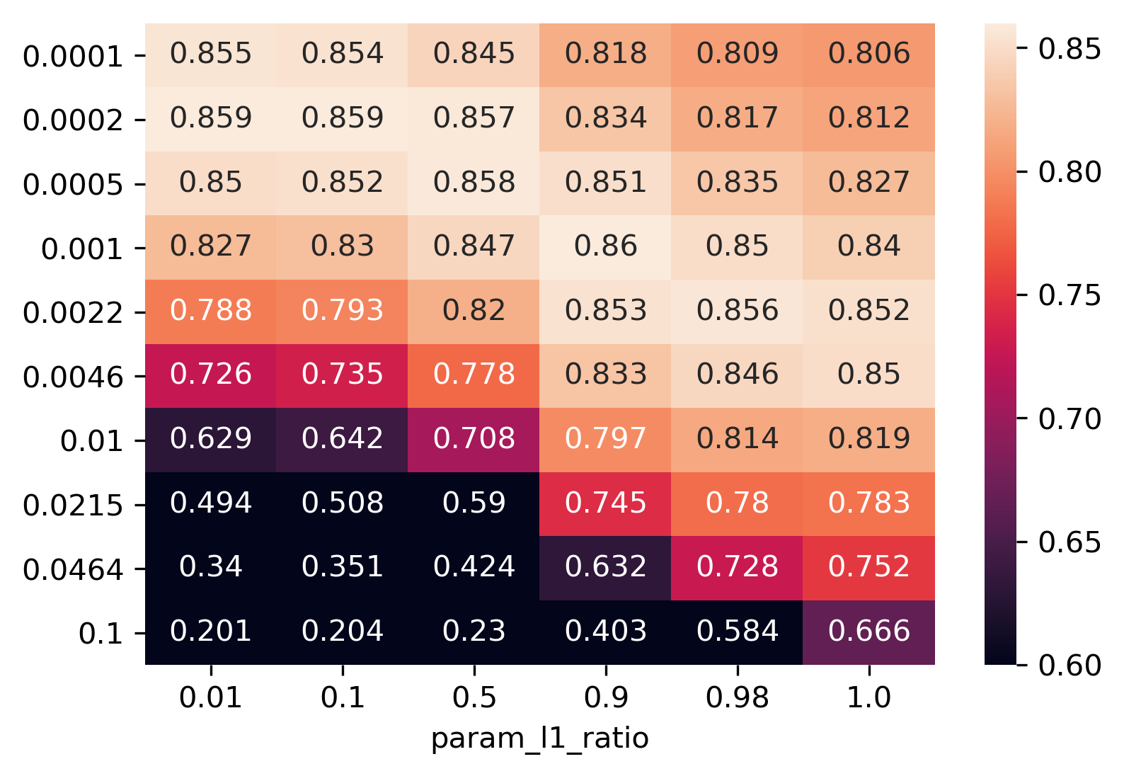
![:scale 60%](images/elasticnet_search.png)
]
???
The way that I like to do it is, here's the grip.cv results.
And I put it in a data frame and then I'll make a pivot
table where the values are test score, the index is one
parameter and the columns are the other parameter. It allows
me to visualize the grid search nicely. This is alpha and
this is l1_ratio and you can see that if the l1_ratio is
pretty high, there are some pretty good results, if you set
the alpha accordingly. So here's like the diagonal of pretty
good things. This is the model that did best. There's a
slight caveat here that right now I did this with
cross-validation and so this is the cross-validation
accuracy. Last time I said, this is not really a good
measure of generalization performance. So here, I searched
way more parameters, I tried like 5 or 10 times as many
models. So it's likely that by chance, I'll get better
results. I didn't do this here in particular, because the
data set is small and very noisy but in practice, if you
want to compare models, you should evaluate it on a test set
and see which of the models actually are better on the test.
One more thing, why this is helpful is if the best value is
on the edge of this graph that means my ranges were too
small. Question is why we're using r square instead of the
squared loss, one of the answers is that's the default in
scikit-learn and the other answer is it's nice to know the
range so you know that perfect prediction is one and you
have some idea of what 0.5 means, the RMSE (the other norm
that you usually use is the RMSE) depends on the scale of
the output. So for example for the housing prices, it might
be interesting to see what is the standard error in terms of
dollars. If you want, like something that is in the units of
the output, RMSE is good or mean absolute error might even
be better. If you want something that is independent of the
units of the output r square is pretty good because you know
it's going to be between zero and one and it's measure
something like the correlation and so if it's like 0.9, you
know it’s a pretty good model. If my RMSE is 10,000 I don't
know if have a good model or a bad model depends on what the
range of the outputs is. The last thing I want to talk about
today is this was basically changing the regularization
parts. The two most times regularization we looked at is
Ridge which is L2 penalty, Lasso which is an L1 penalty and
combining two of them which is Elastic Net. So now I want to
talk about changing the first part, which was the squared
loss of the predictions, basically.

---
class: center, middle

# Notebook: Linear Models for Regression