class: center, middle  ### Intermediate Machine learning with scikit-learn # Linear Models for Classification Andreas C. Müller Columbia University, scikit-learn .smaller[https://github.com/amueller/ml-workshop-2-of-4] --- class: center, middle # Linear models for <strong>binary</strong> classfication ??? We'll first start with linear models for binary classification, so if there are only two classes. That makes the models much easier to understand. --- .center[ 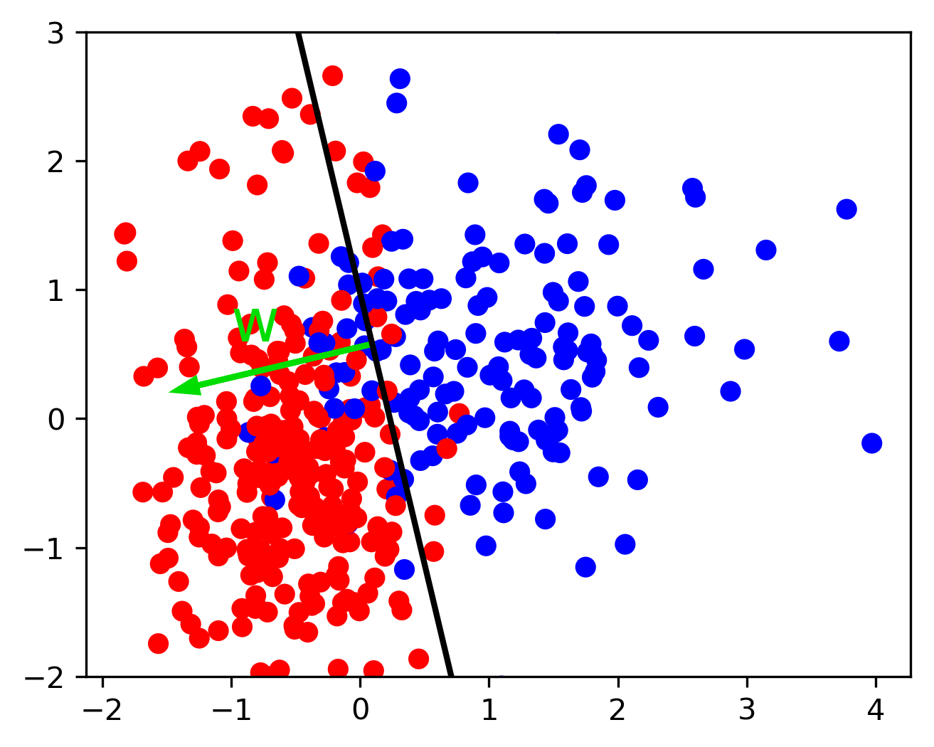 ] $$\hat{y} = \text{sign}(w^T \textbf{x} + b) = \text{sign}\left(\sum\limits_{i}w_ix_i + b\right)$$ ??? Similar to the regression case, basically all linear models for classification have the same way to make predictions. As with regression, they compute an inner product of a weight vector w with the feature vector x, and add some bias b. The result of that is a real number, as in regression. For classification, however, we only look at the sign of the result, so whether it is negative or positive. If it's positive, we predict one class, usually called +1, if it's negative, we predict the other class, usually called -1. If the result is 0, by convention the positive class is predicted, but because it's a floating point number that doesn't really happen in practice. You'll see that sometimes in my notation I will not have a $b$. That's because you can always add a constant feature to x to achieve the same effect (thought you would then need to leave that feature out of the regularization). So when I write $w^Tx$ without a $b$ assume that there is a constant feature added that is not part of any regularization. Geometrially, what the formula means is that the decision boundary of a linear classifier will be a hyperplane in the feature space, where w is the normal vector of that plane. In the 2d example here, it's just a line separating red and blue. Everything on the right hand side would be classified as blue by this classifier, and everything on the left-hand side as red. Questions? So again, the learning here consists of finding parameters w and b based on the training set, and that is where the different algorithms differ. There are quite a lot of algorithms out there, and there are also quite a lot in scikit-learn, but we'll only discuss the most common ones. The most straight-forward way to approach finding w and b is to use the framework of empirical risk minimization that we talked about last time, so finding parameters that minimize some loss o the training set. Where classification differs quite a bit from regression is on how we want to measure misclassifications. --- # Picking a loss? $$\hat{y} = \text{sign}(w^T \textbf{x} + b)$$ `$$\min_{w \in ℝ^{p}, b \in \mathbb{R}} \sum_{i=1}^n 1_{y_i \neq \text{sign}(w^T \textbf{x} + b)}$$` .center[ 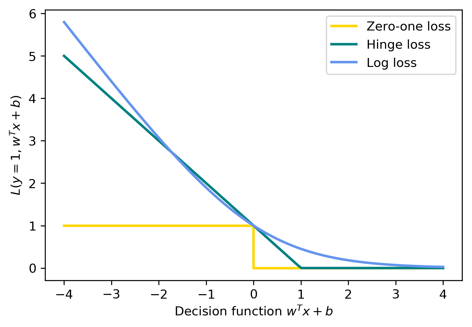 ] ??? So we need to define a loss function for given w and b that tell us how well they fit the training set. Obvious Idea: Minimize number of misclassifications aka 0-1 loss but this loss is non-convex, not continuous and minimizing it is NP-hard. So we need to relax it, which basically means we want to find a convex upper bound for this loss. This is not done on the actual prediction, but on the inner product $w^T x$, which is also called the decision function. So this graph here has the inner product on the x axis, and shows what the loss would be for class 1. The 0-1 loss is zero if the decision function is positive, and one if it's negative. Because a positive decision function means a positive predition, means correct classification in the case of y=1. A negative prediction means a wrong classification, which is penalized by the 0-1 loss with a loss of 1, i.e. one mistake. The other losses we'll talk about are mostly the hinge loss and the log loss. You can see they are both upper bounds on the 0-1 loss but they are convex and continuous. Both of these losses care not only that you make a correct prediction, but also "how correct" your prediction is, i.e. how positive or negative your decision function is. We'll talk a bit more about the motivation of these two losses, starting with the logistic loss. --- # Logistic Regression .left-column[ $$\log\left(\frac{p(y=1|x)}{p(y=-1|x)}\right) = w^T\textbf{x} + b$$ $$p(y=1|\textbf{x}) = \frac{1}{1+e^{-w^T\textbf{x} -b }}$$ `$$\min_{w \in ℝ^{p}, b \in \mathbb{R}} \sum_{i=1}^n \log(\exp(-y_i(w^T \textbf{x}_i + b)) + 1)$$` $$\hat{y} = \text{sign}(w^T\textbf{x} + b)$$ ] .right-column[ 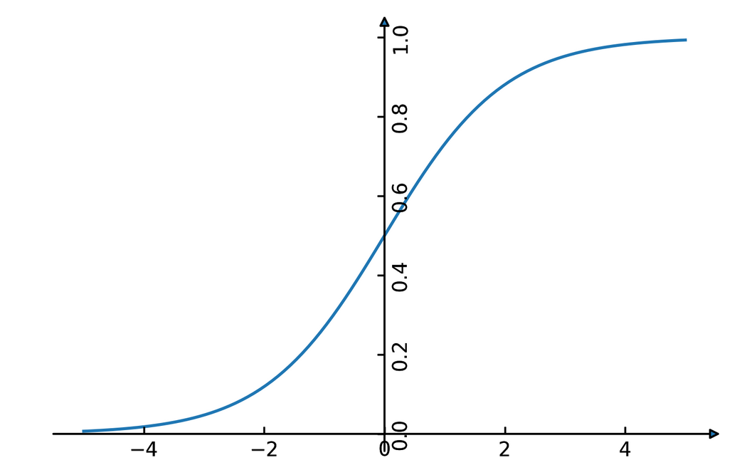] ??? Logistic regression is probably the most commonly used linear classifier, maybe the most commonly used classifier overall. The idea is to model the log-odds, which is log p(y=1|x) - log p(y=0|x) as a linear function, as shown here. Rearranging the formula, you get a model of p(y=1|x) as 1 over 1 + ... This function is called the logistic sigmoid, and is drawn to the right here. Basically it squashed the linear function $w^Tx$ between 0 and 1, so that it can model a probability. Given this equation for p(y|x), what we want to do is maximize the probability of the training set under this model. This approach is known as maximum likelihood. Basically you want to find w and b such that they assign maximum probability to the labels observed in the training data. You can rearrange that a bit and end up with this equation here, which contains the log-loss as seen on the last slide. The prediction is the class with the higher probability. In the binary case, that's the same as asking whether the probability of class 1 is bigger or smaller than .5. And as you can see from the plot of the logistic sigmoid, the probability of the class +1 is greater than .5 exactly if the decision function $w^T x$ is greater than 0. So predicting the class with maximum probability is the same as predicting which side of the hyperplane given by w we are on. Ok so this is logistic regression. We minimize this loss and get a w which defines a hyper plane. But if you think back to last time, this is only part of what we want. This formulation tries to fit the training data, but it doesn't care about finding a simple solution. --- # Penalized Logistic Regression `$$\min_{w \in ℝ^{p}, b \in \mathbb{R}}C \sum_{i=1}^n\log(\exp(-y_i(w^T \textbf{x}_i + b )) + 1) + ||w||_2^2$$` `$$\min_{w \in ℝ^{p}, b \in \mathbb{R}}C \sum_{i=1}^n\log(\exp(-y_i (w^T \textbf{x}_i + b)) + 1) + ||w||_1$$` - C is inverse to alpha (or alpha / n_samples) ??? - Both versions strongly convex, l2 version smooth (differentiable). - All points contribute to $w$ (dense solution to dual). So we can do the same we did for regression: we can add regularization terms using the L1 and L2 norm. The effects are the same as for regression: both push the coefficients towards zero, but the l1 norm encourages coefficients to be exactly zero, for the same reasons we discussed last time. You could also use a mixed penalty to get something like the elasticnet. That's not implemented in the logisticregression class in scikit-learn right now, but it's certainly a sensible thing to do. Here I used a slightly different notation as last time, though. I'm not using alpha to multiply the regularizer, instead I'm using C to multiply the loss. That's mostly because that's how it's done in scikit-learn and it has only historic reasons. The idea is exactly the same, only now C is 1 over alpha. So large C means heavy weight to the loss, means little regularization, while small C means less weight on the loss, means strong regularization. Depending on the model, there might be a factor of n_samples in there somewhere. Usually we try to make the objective as independent of the number of samples as possible in scikit-learn, but that might lead to surprises if you're not aware of it. Some side-notes on the optimization problem: here, as in regression, having more regularization makes the optimization problem easier. You might have seen this in your homework already, if you decrease C, meaning you add more regularization, your model fits more quickly. One particular property of the logistic loss, compared to the hinge loss we'll discuss next is that each data point contributes to the loss, so each data point has an effect on the solution. That's also true for all the regression models we saw last time. --- # Effect of regularization .center[ 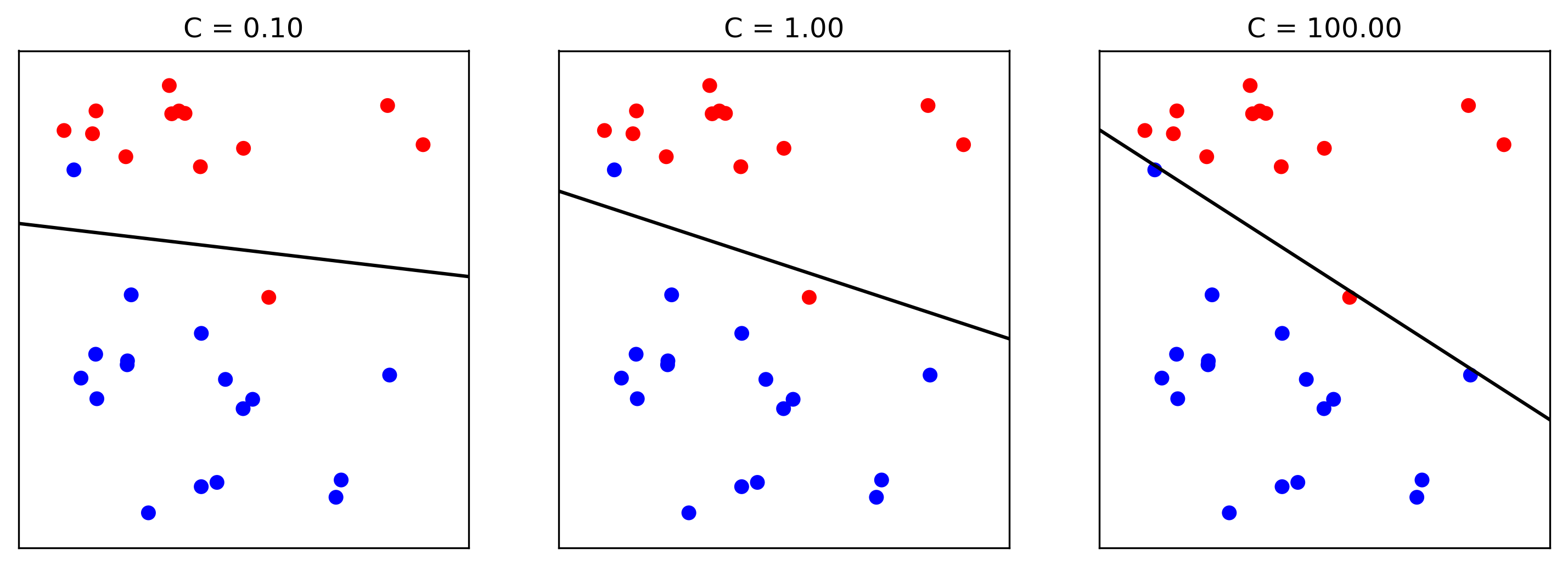 ] - Small C (a lot of regularization) limits the influence of individual points! ??? So I spared you with coefficient plots, because they looks the same as for regression. All the things I said about model complexity and dependency on the number of features and samples is as true for classification as it is for regression. There is another interesting way to thing about regularization that I found helpful, though. I'm not going to walk through the math for this, but you can reformulate the optimization problem and find that what the C parameter does is actually limit the influence of individual data points. With very large C, we said we have no regularization. It also means individual data points can have basically unlimited influence, as you can see here. There are two outliers here, which basically completely tilt the decision boundary. But if we decrease C, and therefore increase the regularization, what happens is that the influence of these outlier points becomes limited, and the other points get more influence. --- #Max-Margin and Support Vectors .center[ 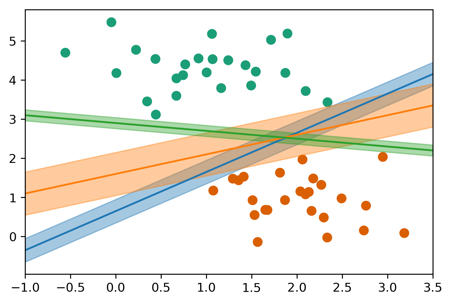 ] ??? A point is within the margin if 〖y_i w〗^T x is smaller than one. That means if you have a smaller w, you basically have a smaller margin given that you're on the correct side. If you're on the wrong side, you'll have always have a loss. If you're in the correct side, if you're w^x is small, then you also have a loss. --- class: center #Max-Margin and Support Vectors `$$ \min_{w \in \mathbb{R}^p, b \in \mathbb{R}} C \sum_{i=1}^n \max(0, 1 - y_i (w^T\mathbf{x} + b)) + ||w||^2_2 $$` $$\text{Within margin} \Leftrightarrow y_i(w^T x + b)< 1$$ Smaller $w \Rightarrow$ larger margin --- class: center #Max-Margin and Support Vectors .left-column[ 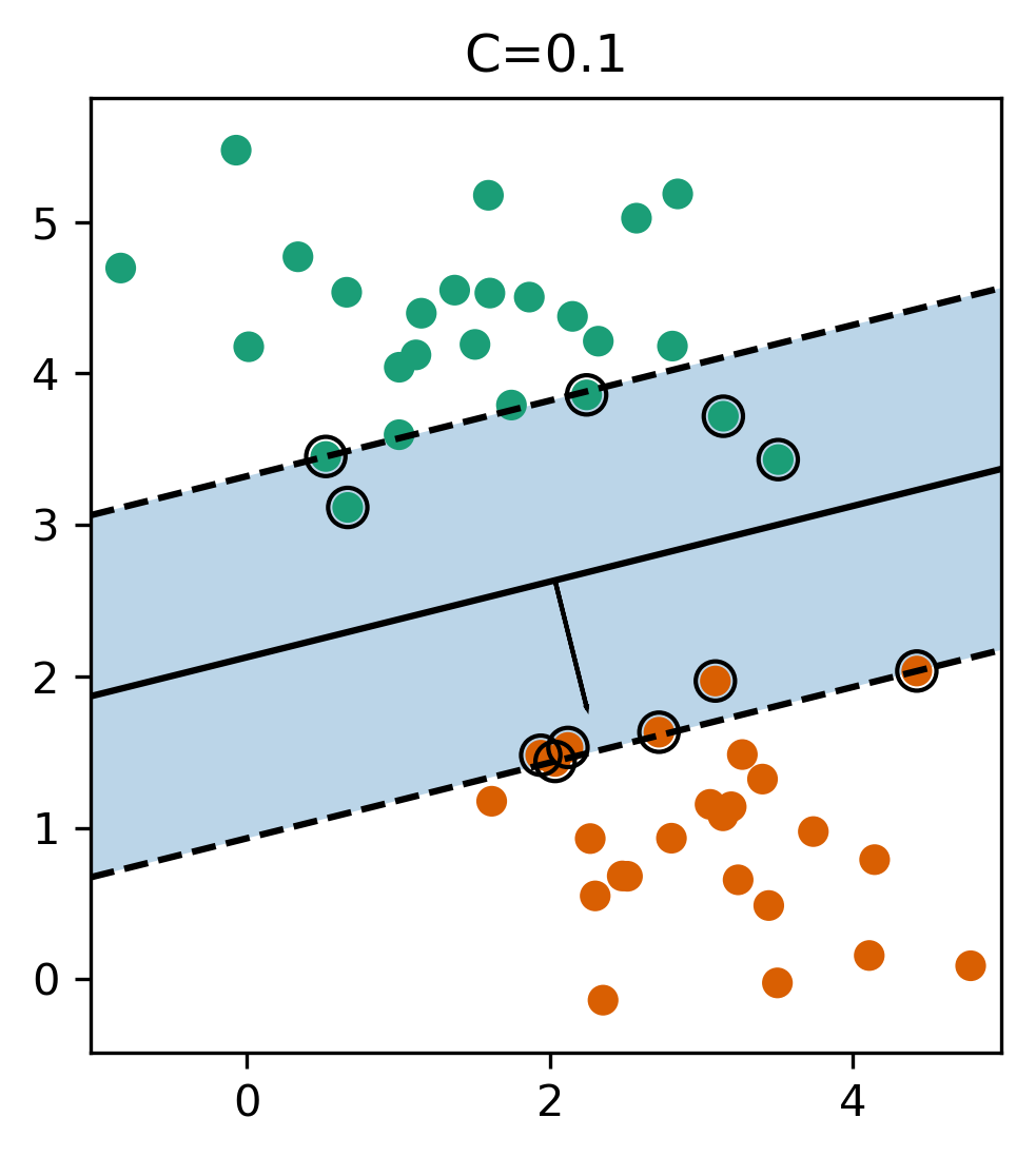 ] .right-column[ 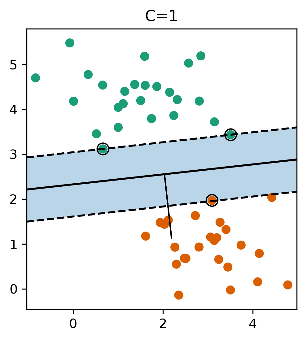 ] ??? Here are two examples on the same dataset. Where I learned linear support vector machine with c-0.1, and c=1. With c=0.1, you have a wider margin. There are points inside the margin and all the points inside the margin are support vectors which contribute to the solution. Points that are outside of the margin and on the correct side doesn't contribute to the solution. These points are sort of classified correctly, not when they’re ignored. The normal vector is w and basically, the size of the margin is the inverse of the length of w. C=0.1 means I have less emphasis on the data fitting and more emphasis on the shrinking w. This will lead to a smaller w. If I have larger C that means less regularization, which will lead to a larger W, larger W means a smaller margin. So there are fewer points here, they are inside the margin and therefore, fewer support vectors. More regularization usually means a larger margin but more points inside the margin. Also, more support vectors mean there are more data points that actually influence the solution. --- # (soft margin) linear SVM .larger[ `$$\min_{w \in ℝ^{p}, b \in \mathbb{R}}C \sum_{i=1}^n\max(0,1-y_i(w^T \textbf{x}_i + b)) + ||w||_2^2$$` `$$\min_{w \in ℝ^{p}, b \in \mathbb{R}}C \sum_{i=1}^n\max(0,1-y_i(w^T \textbf{x}_i + b))+ ||w||_1$$` ] ??? - Both versions strongly convex, neither smooth. - Only some points contribute (the support vectors) to $w$ (sparse solution to dual). Moving from logistic regression to linear SVMs is just a matter of changing the loss from the log loss to the hinge loss. The hinge-loss is defined as ... And we can penalize using either l1 or l2 norm, or again, in principle also elastic net. This formulation with the hinge loss doesn't really make sense without the penalty, because of the formulation of the hinge loss. What this loss says is basically "if you predict the right class with a margin of 1, there is no loss". Otherwise the loss is linear in the decision function. So you need to be on the right side of the hyperplane by a given amount, and then there is no more loss. That's the reason you need the penalty, for the 1 to make sense. Otherwise you could just scale up $w$ to make it far enough on the right side. But the regularization penalizes growing $w$. The hinge loss has a kink, same as the l1 norm, and so it's not a smooth optimization problem any more, but that's not really a big deal. What's interesting is that all the points that are classified correctly with a margin of at least 1 have a loss of zero, and so they don't influence the solution any more. All the point that are not classified correctly by this margin are the ones that do influence the solution and they are called the support vectors. FIXME graph of not influencing the solution? --- class: center # Logistic Regression vs SVM .compact[ `$$\min_{w \in ℝ^{p}, b \in \mathbb{R}}C \sum_{i=1}^n\log(\exp(-y_i(w^T \textbf{x}_i+b)) + 1) + ||w||_2^2$$` `$$\min_{w \in ℝ^{p}, b \in \mathbb{R}}C \sum_{i=1}^n\max(0,1-y_i(w^T \textbf{x}_i + b)) + ||w||_2^2$$`  ] ??? So this is the main difference between logistic regression and linear SVMs: Does it penalize misclassifications according to the green line, or according to the blue line? In practice it doesn't make a big difference. --- # SVM or LogReg? .center[ 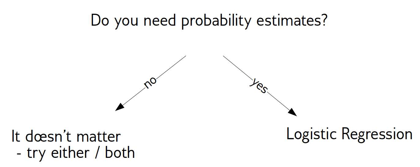 ] - Need compact model or believe solution is sparse? Use L1 ??? So which one of them should you use? If you need probability estimates, you should use logistic regression. If you don't, you can pick either, and it doesn't really matter. Logistic regression can be a bit faster to optimize in theory. If you're in a setting where there's many more feature than samples, it might make sense to use linear SVMs and solve the dual, but you can actually solve either of the problems in the dual, and we'll talk about what that means in practice in a little bit. --- class: center, middle # Multiclass classification ??? Ok, so I think that's enough on the two loss functions and regularization, and hopefully you have a bit of a feel for how these two classifiers work, and also an understanding that they are in fact quite similar in practice. Next I want to look at how to go from binary classification to multi-class classification. Basically there is a simple but hacky way, and there's a slightly more complicated but theoretically sound way. --- class: center # Reduction to Binary Classification # One Vs Rest For 4 classes: 1v{2,3,4}, 2v{1,3,4}, 3v{1,2,4}, 4v{1,2,3} In general: n binary classifiers - each on all data ??? Let's start with One vs Rest. here, we learn one binary classifier for each class against the remaining classes. So let's say we have 4 classes, called 1 to 4. First we learn a binary classifier of the points in class 1 vs the points in the classes 2, 3 and 4. Then, we do the same for class 2, and so on. The way we end up building as many classifiers as we have classes. --- class: spacious # Prediction with One Vs Rest "Class with highest score" $$\hat{y} = \text{arg}\max_{i \in Y} \textbf{w}^T_i\textbf{x} + b_i$$ ??? To make a prediction, we compute the decision function of all classifiers, say 4 in the example, on a new data point. The one with the highest score for the positive class, the single class, wins, and that class is predicted. It's a little bit unclear why this works as well as it does. Maybe there's some papers about that now, but I'm not So in this case we have one coefficient vector w and one bias b for each class. --- # One vs Rest Prediction .center[ 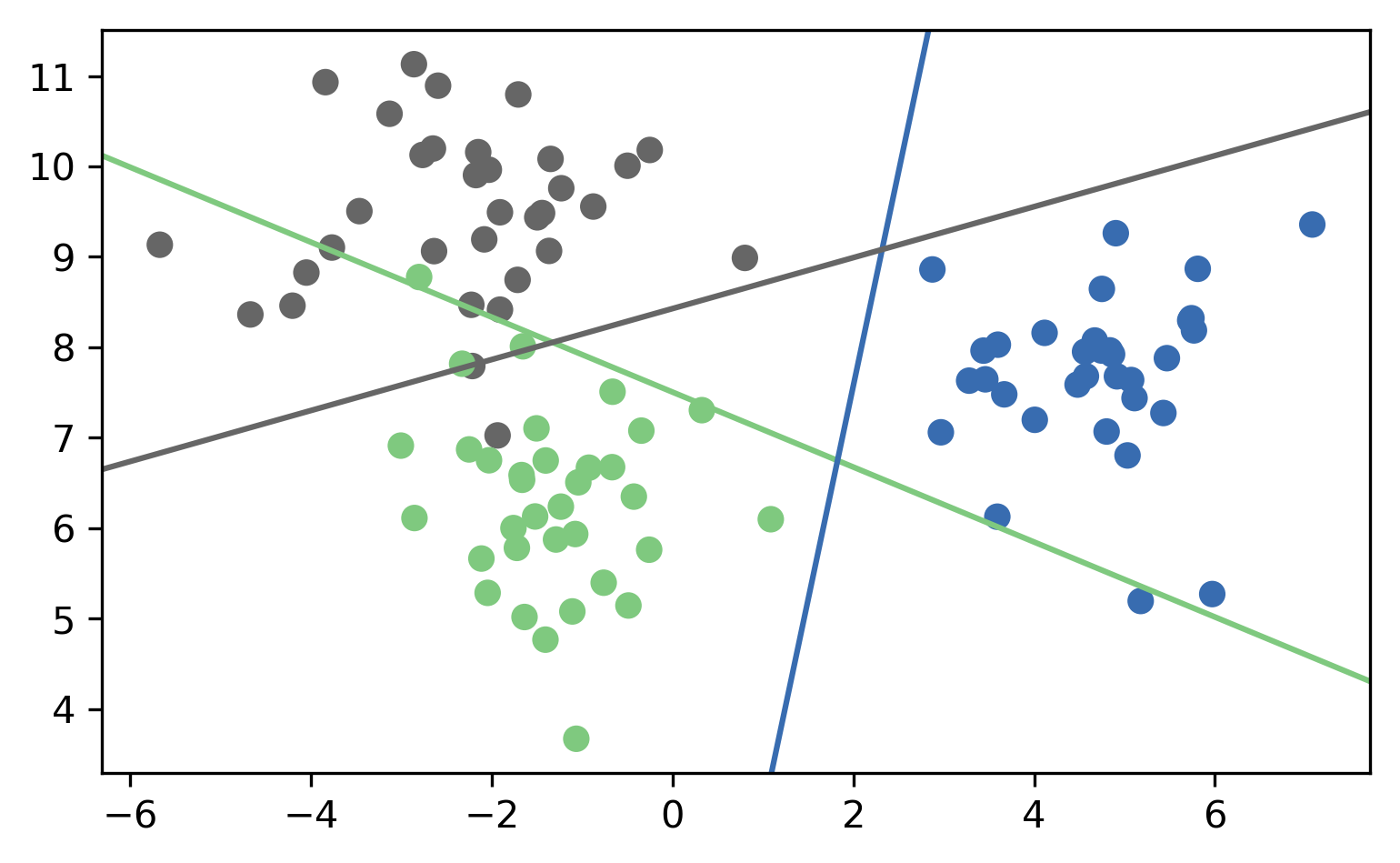 ] ??? Here is an illustration of what that looks like. Unfortunately it's a bit hard to draw 4 classes in general position in 2 dimensions, so I only used 3 classes here. So each class has an associated coefficient vector and bias, corresponding to a line. The line tries to separate this class from the other two classes. # Fixme draw ws? --- # One vs Rest Prediction .center[ 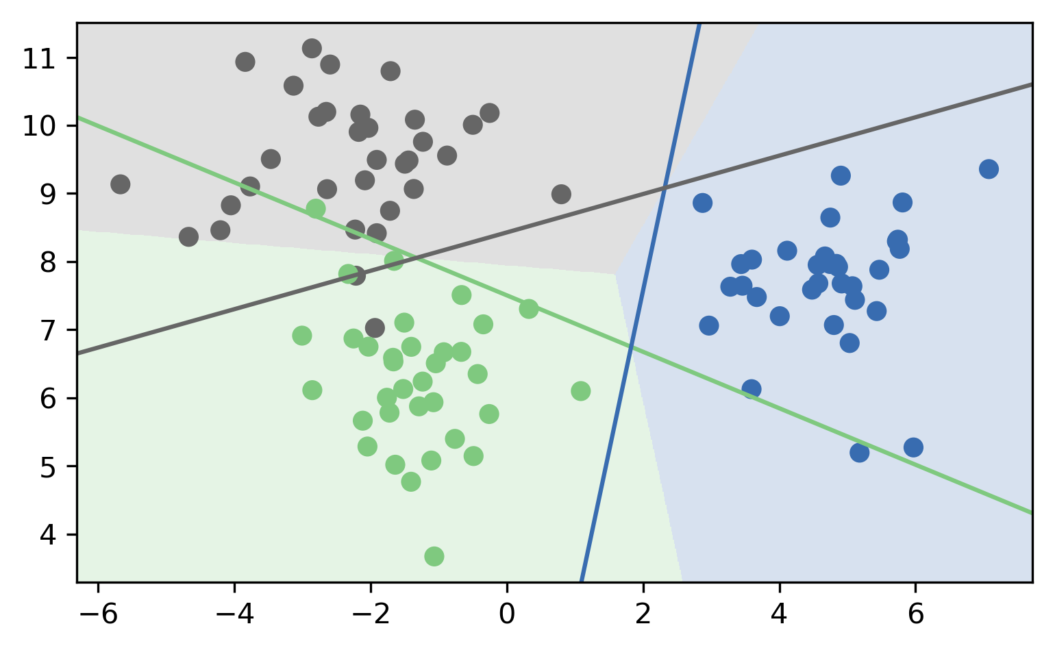 ] ??? Here are the decision boundaries resulting from the these three binary classifiers. Basically what they say is that the line that is closest decides the class. What you can not see here is that each of the lines also have a magnitude associated with them. It's not only the direction of the normal vector that matters, but also the length. You can think of that as some form of uncertainty attached to the line. --- # Multinomial Logistic Regression Probabilistic multi-class model: `$$p(y=i|x) = \frac{e^{\textbf{w}_i^T\textbf{x} + b_i}}{\sum_{j=1}^k e^{\textbf{w}_j^T\textbf{x} + b_j}}$$` `$$\min_{w \in ℝ^{pk}, b \in \mathbb{R}^k} -\sum_{i=1}^n \log(p(y=y_i|x_i, w, b))$$` $$\hat{y} = \text{arg} \max_{i=1,...,k} \textbf{w}^T_i\textbf{x} + b_i$$ - Same prediction rule as OvR ! ??? The binary logistic regression case can be generalized to multinomial logistic regression, in which we model the probability that i is one of the classes using this formula, which is also known as softmax. The probability is proportional to e to the minus $w^t x$ which is the same as in the binary case. But now we need to normalize it so that the sum over all classes is one. So we just divide it by this sum. --- class: center, middle # Notebook: Linear Models for Classification