Trees and Forests

![:scale 40%](images/sklearn_logo.png)

### Intermediate Machine learning with scikit-learn

# Trees and Forests

Andreas C. Müller

Columbia University, scikit-learn

???
FIXME bullet points!
animation searching for split in tree?
categorical data split?
predition animation tree?
min impurity decrease missing
extra tree: only one thereshold per feature?

---
class: spacious, middle
# Why Trees?
???
Trees are really very powerful models both for
classification and regression, they're very commonly used.
Trees are very popular in the industry. Only beaten by
deep neural networks. Tree-based models are one of the main
tools in the toolbox of most machine learning practitioners.

Trees really don't care about the scale of the data so you
don't really have to do a lot of preprocessing. Trees don't
care about the distribution of your data. There are versions
of trees that can deal with categorical variables and with
missing values.  By combining multiple trees you can build
stronger models.
- Very powerful modeling method – non-linear!
- Doesn’t care about scaling of distribution of data!
- “Interpretable”
- Basis of very powerful models!
- add stacking classifier from PR?
---

# Idea: series of binary questions
.center[
![:scale 70%](images/tree_illustration.png)
]
???
Binary classification trees are binary trees, where each
node corresponds to a question asked about the data. This
example is a fictional task where you want to distinguish
hawks, penguins, dolphins, and bears. You ask a series of
binary questions that will lead to which animal it might be.

Depending on what the answer is for a particular question,
you could ask another question. This way you can narrow it
down for possible outcomes. Usually, when we are doing
classification we have continuous features and so the
questions are thresholds on single features.

---
# Building Trees

.left-column[
![:scale 100%](images/tree_building_iteration_1.png)
<br />
<br />
Continuous features:
 - “questions” are thresholds on single features.
 - Minimize impurity
]
.right-column[
![:scale 100%](images/tree_building_iteration_2.png)

![:scale 100%](images/tree_building_iteration_9.png)
]

???
Here is an example of a tree with depth one, that's
basically just thresholding a single feature. In this
example, the question being asked is, is X1 less than or
equal to 0.0596. The boundary between the 2 regions is the
decision boundary. The decision for each of the region would
be the majority class on it. This decision tree of depth one
would classify everything that is below the horizontal line
as class red since there are more red points (32>2) and
everything above as blue since there are more blue points
(48>18).

The way this threshold was chosen, the way that tree of
depth one was learned was to find the best feature and the
best threshold to minimize impurity. Which means it tries to
make the resulting subsets, the top half and the bottom half
here, to be as pure as possible (to consist mostly of one
class)

Basically, we're searching over all possible features and
all possible thresholds. Possible thresholds are all values
of the feature that we're observing. So I would start
iterating over the first feature and for the first feature,
I would look at all possible thresholds and see if this is a
good question to ask, i.e. is this a good way to split the
data set into two classes.

If you search over all possible features, then the best
split is found. Once we find this split, we can then
basically apply this algorithm recursively to the two areas
that the split created. For top area here, we can ask what
the best feature is and what the best threshold for this
feature is to make the resulting regions as pure as
possible.

Here in the bottom, it asks is X0 less or equal than minus
0.4? The model will predict accordingly, either blue or red.
If only one class remain after a split, the tree will not
add any splits since the regions have become pure. Each node
corresponds to a split and the leaves correspond to regions.
All tree building algorithms start greedily building a tree,
so they don't really go back and revisit because it would be
too computationally expensive.
Does the layout look okay??
---

# Criteria (for classification)
 - Gini Index:

`$$H_\text{gini}(X_m) = \sum_{k\in\mathcal{Y}} p_{mk} (1 - p_{mk})$$`

- Cross-Entropy:

`$$H_\text{CE}(X_m) = -\sum_{k\in\mathcal{Y}} p_{mk} \log(p_{mk})$$`

$X_m$ observations in node m

$\mathcal{Y}$ classes

$p_{m\cdot}$ distribution over classes in node m
???
 For classification, there are two common criteria to
 preserve the purity of the leaf. One is called the Gini
 Index and the other one is Cross-Entropy.

Gini Index works well in practices. Cross-Entropy is the
entropy of the distribution over classes. You want to
minimize the entropy over the classes, you want to have a
very spike distribution in the classes, you want mostly to
be one class and less of the others so that the trees are
very certain about what the class is for each leaf.
---

# Prediction

???
To make a prediction, I traverse the tree I ask all the
questions in the node that I encounter and then I can
predict the majority class in the leaf. One thing that's
nice about this is this prediction is really, really fast
since this tree is not very deep.
 - Traverse tree based on feature tests
 - Predict most common class in leaf

---

# Regression trees

`$$\text{Prediction: } \bar{y}_m = \frac{1}{N_m} \sum_{i \in N_m} y_i $$`

Mean Squared Error:
`$$ H(X_m) = \frac{1}{N_m} \sum_{i \in N_m} (y_i - \bar{y}_m)^2 $$`

Mean Absolute Error:
`$$ H(X_m) = \frac{1}{N_m} \sum_{i \in N_m} |y_i - \bar{y}_m| $$`

???
You can do the same thing also for regression. In
regression, the prediction is usually the mean over the
target targets in a leaf. The impurity criteria that I
minimized is usually the mean squared error. Basically, you
look at how good of a prediction is the mean if I split like
this. For each possible split, you can compute the mean for
the two resulting nodes and you compute how well the mean in
this leaf predicts.

You can use the mean absolute error, if you want it to be
more robust outliers then you don’t penalize with the square
norm, you only penalize with the L1 norm.

One thing about the regression trees is that they have more
tendency to get very deep if you don't restrict them.
Because usually in regression, all targets are distinct,
they’re distinct float numbers. So if you want all leaves to
be pure, then all of these will have only one node in them,
unless you have a special case where you have equal flow
numbers as a target, which is not common.

Another thing that's really nice about trees is that you can
visualize them and you can look at them, and you can
possibly even explain to your boss what they mean.
 - Without regularization / pruning:
 - Each leaf often contains a single point to be “pure”

---

# Visualizing trees with sklearn

.smaller[
```python
from sklearn.datasets import load_breast_cancer
cancer = load_breast_cancer()
X_train, X_test, y_train, y_test = train_test_split(cancer.data,cancer.target,
                                                    stratify=cancer.target,
                                                    random_state=0)

from sklearn.tree import DecisionTreeClassifier
tree = DecisionTreeClassifier(max_depth=2)
tree.fit(X_train, y_train)

```
]

???
The first way to visualize tree in scikit-learn is a little
bit tricky. The second one is a one I hacked.

I'm going to use the breast cancer data center, which does
the classification of breast tissues. So trees can do much
more complicated things than multiclass. For the ease of
visualization, I'm going to do binary.

I can build the decision tree classifier, and there's a
method in scikit-learn called export _graphviz, which is
basically a file format and the layout engine for showing
graphs.

So you can take the tree, the estimator that’s the tree. You
can also give it the feature names if you want. You can
either write this to a file, or you can get back to string
in this dot language. And that's what it looks like. This is
a tree of depth 2 and I gave it the feature names.

---
# Visualizing trees with sklearn

```python
from sklearn.tree import plot_tree
tree_dot = plot_tree(tree, feature_names=cancer.feature_names)
```
.center[
![:scale 80%](images/mpl_tree_plot.png)
]

???
The other thing that I like to use which is easier is this
pull request or there’s a gist that you download, it’s a
single file called the tree_plotting. And that uses math
plot to plot the trees.

Here, at the top you can see the test, then you can see the
criteria, then the number of samples in this node and then
which class the samples belong to. In the original breast
cancer dataset, the top node corresponds to the whole
dataset. The tree gets purer and purer as you move down the
tree.
---
class:some-space

# Parameter Tuning

- Pre-pruning vs post-pruning

- Pre-pruning: Limit tree size (pick one, maybe two):

- max_depth

- max_leaf_nodes

- min_samples_split

- min_impurity_decrease

- ...
???
  I want to talk a little bit about the different parameters
  that you can choose. Most of the tree growing algorithms
  are greedy. There are two ways to restrict the growth of
  the tree after you train them. There are pre-pruning and
  post-pruning.

In pre-pruning, you restrict while you're growing. In
post-pruning, you build the whole tree (greedily) and then
you possibly merge notes. So you possibly undo sort of bad
decisions that you made, but you don't restructure the tree.

In scikit-learn right now, there's only pre-pruning. The
most commonly used criteria are the maximum depth of the
tree, the maximum number of leaf nodes, the minimum samples
in a node split and minimum decrease impurity.
---
class:spacious

# No pruning
.center[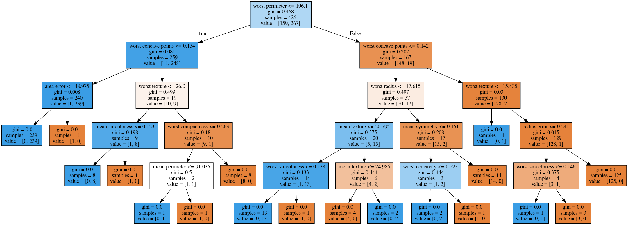
![:scale 100%](images/no_pruning.png)
]
???

Here’s the full tree for the same dataset.
---
class:spacious

# max_depth = 4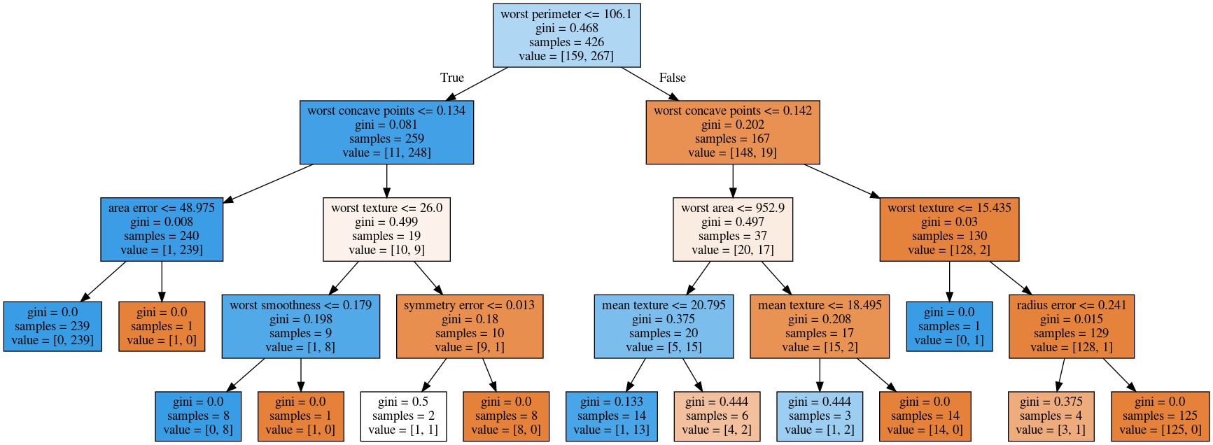

???
Maximum depth of the tree restricted to 4. This is like a
very simple way. If you are actually building just a single
decision tree, this might not be the best way because for
example, here you split away the single point which might
not be great and other leaves are very mixed. So you can't
make a good prediction here. Since it puts the same depth
limit on everywhere in the tree, this is not very fine
grained.

What it does is it means that your predictions will be very
fast because you never have to go very deep in the tree. It
also makes the tree size very small. If you built a lot of
trees, you might get issues with the RAM. If you have a lot
of very deep trees, they will at some point be bigger than
your RAM, and you'll run into troubles, or if they're very
deep, it might be very slow to predict at some point. So
this is a way to restrict how much memory and how much
prediction time you're willing to give.
---

# max_leaf_nodes = 8
.center[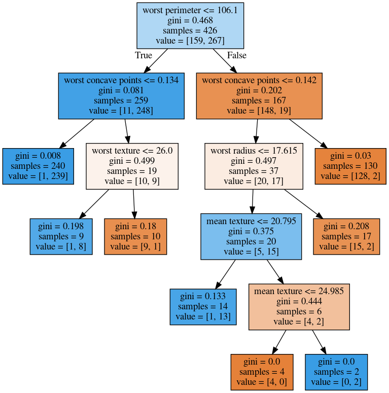
![:scale 50%](images/max_leaf_nodes_8.png)
]

???
If you use max_leaf_nodes, it will always put the one that
has the greatest impurity decrease first. You can see that
in different parts of the trees, there's different depth. It
will prioritize the ones that decrease the impurity the
most.
---
class:spacious

# min_samples_split = 50
.center[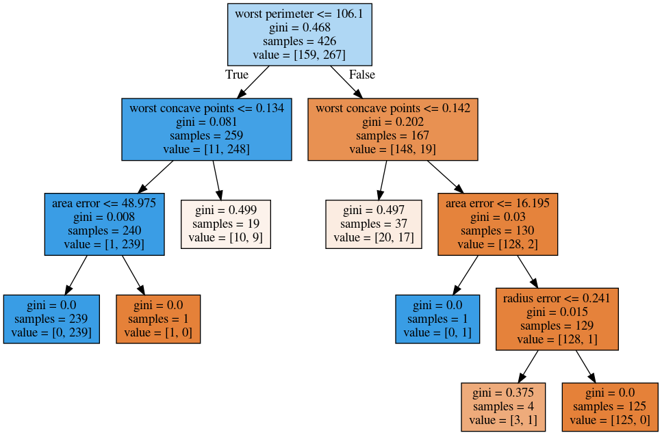
![:scale 70%](images/min_samples_split_50.png)
]

???
Min_samples_split is quite simple, it just says only split
nodes that have this many samples on them. What I don't like
about this criterion set here, for example, it splits off a
single point, which I don't think is really great, because
it's not going to improve the prediction very much.

So both the max leaf nodes and the minimum impurity decrease
will allow you to basically get rid of these very small
leaves that don't really add anything to the prediction.

Impurity decrease will only make splits that decrease the
impurity by X amount.

If you want to tune this, you pick one of these and then you
just tune this one parameter.
---

.smaller[
```python
from sklearn.model_selection import GridSearchCV
param_grid = {'max_depth':range(1, 7)}
grid = GridSearchCV(DecisionTreeClassifier(random_state=0),
                    param_grid=param_grid, cv=10)
grid.fit(X_train, y_train)
```
]
.center[
![:scale 70%](images/grid_max_depth.png)
]

???
So for example, if you want to tune max depth and restricted
the depth of the tree. So run a grid search over max depth
and you can do the parameter curves as we did before and you
can see that maybe depth of five is good on this dataset.

Again, you can see the typical curve with the more
complexity you allow in your classifier, the better you get
the training set, but possibly you overfit on a test set.
So, here, you could say maybe it's overfitting a little bit,
but it's not very visible.
---
.smaller[
```python
from sklearn.model_selection import GridSearchCV
param_grid = {'max_leaf_nodes':range(2, 20)}
grid = GridSearchCV(DecisionTreeClassifier(random_state=0),
                    param_grid=param_grid, cv=10)
grid.fit(X_train, y_train)
```
]
.center[
![:scale 70%](images/grid_max_leaf_nodes.png)
]

???
Here is if you tune a maximum number of leaf nodes, you can
see it’s slightly more overfitting happening but generally,
there's not a big difference on this toy dataset between
building the full tree or having a smaller tree. Obviously,
if you have a small tree, predictions are going to be faster
and need less memory to store and you can explain it better.

So the thing with being able to explain is, if you have a
tree up depth 14, then it's not really explainable anymore,
no human can look at all of this and say “Oh, I understand
exactly what's going on”. If you have 8 leaves, it's a very
good chance you can draw this, and you can think about it,
and you can understand that.

I wouldn't really say trees are interpretable but small
trees are interpretable. So that's also the reason why you
might want to restrict the rows of the tree. So you can
easily communicate and easily explained.
---
# Cost Complexity Pruning
.padding-top[
.larger[
$$  R_\alpha(T) = R(T) + \alpha|T| $$
]
]

$R(T)$ is total leaf impurity

$|T|$ is number of leaf nodes

$\alpha$ is free parameter.
---

.smaller[
```python
from sklearn.model_selection import GridSearchCV
param_grid = {'ccp_alpha': np.linspace(0., 0.03, 20)}
grid = GridSearchCV(DecisionTreeClassifier(random_state=0),
                    param_grid=param_grid, cv=10)
grid.fit(X_train, y_train)
```
]
.center[
![:scale 70%](images/grid_ccp_alpha.png)
]
---
# Efficient pruning
```python
clf = DecisionTreeClassifier(random_state=0)
path = clf.cost_complexity_pruning_path(X_train, y_train)
ccp_alphas, impurities = path.ccp_alphas, path.impurities
```
.center[
![:scale 55%](images/pruning_alpha.png)
]
---
# Best post-pruned vs pre-pruned
.left-column[
## Cost-complexity pruning
![:scale 70%](images/tree_pruned.png)

]
.right-column[
## Max leaf nodes search
![:scale 80%](images/max_leaf_nodes_8.png)
]
---
#Extrapolation
.center[
![:scale 80%](images/ram_prices.png)
]

???
Trees are actually quite similar to nearest neighbors in
some sense because both nearest neighbors and trees pick the
average of their neighbors or delete the neighbors’ votes
(depending on classification or regression)

In KNearest Neighbors or epsilon nearest neighbors, where
you have a radius around the data point in which you look
for neighbors. In trees, you look at the same leaf, and you
basically let the other point in the leaf vote what the
output should be.

Trees are consistent if you give them enough data and they
will eventually learn anything because eventually, they're
just like nearest neighbors. Nearest neighbors are very slow
to predict because you need to compute the distances to all
training points while trees very fast to predict because you
just need to traverse the binary tree. One thing that you
should keep in mind is that both can't extrapolate.
---
#Extrapolation
.center[
![:scale 80%](images/ram_prices_train.png)
]
???
---
#Extrapolation
.center[
![:scale 80%](images/ram_prices_test.png)
]
???
This is the RAM prices in dollar per megabyte historically.
This is an instance of Moore's law. On log scale, it’s
pretty linear because of the ram prices half every 18 months
or something.

Let's say I want to build the prediction model for this. And
I want to build it up to 2000, and I want to make
predictions about the future. Now I'm going to compare a
linear model in a tree-based model.

The linear model, I kind of cheated a little bit because I
did the log transform so that linear model can actually
model it. I didn't restrict the tree model so it'll
basically learn the training data set perfectly.

Now the question is, if I want to do prediction, what are we
going to predict? You probably are not going to be surprised
by the linear prediction but you might be by the tree
prediction.

The tree predicts just a constant and the constant is
basically the last point observed. This is the same thing
that the nearest neighbor base model would do. So if you
want to predict here, basically, you traverse the tree and
you find basically the closest data point to it, the one or
the other data point that is in the same leaf, and the ones
that will share the leaf with are the ones on the very
right. And then it will computer mean of these data points.
And the mean is going to be just the value if the leaf is
pure. If I did like coarser split level, it will tune the
mean of all of these, but it’ll always compute the mean of
some data points on the training set. So it'll never be able
to predict these values that are not seen in a training set.

In practice, this is usually not really a big issue. For
example, if you want to do like extrapolation like this, you
could instead of trying to predict the value, you could use
the tree to predict the difference to the last day or to the
last year or something like this, and then it would work.
But it's definitely something you should keep in mind.
Basically, outside of where you’ve observed training data,
it'll just be a constant prediction. Basically falling back
to what it was last seen. That might be a little bit
surprising sometimes. Generally, extrapolation in machine
learning is hard. And if you need to extrapolate, there's a
chance you're not going to be able to do with any model. But
in particular, for tree-based and nearest neighbor based
models, you should keep in mind that they can't do that.
---
class:spacious
# Relation to Nearest Neighbors
- Predict average of neighbors – either by k, by epsilon ball or by leaf.
- Trees are much faster to predict.
- Both can’t extrapolate
???
FIXME plots
---

# Instability

.left-column[
.tiny-code[
```python
X_train, X_test, y_train, y_test = train_test_split(
    iris.data, iris.target, stratify=iris.target, random_state=0)
tree = DecisionTreeClassifier(max_leaf_nodes=6)
tree.fit(X_train, y_train)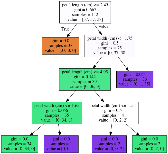
```
]
![:scale 70%](images/instability_1.png)
]
.right-column[
.tiny-code[```python
X_train, X_test, y_train, y_test = train_test_split(
    iris.data, iris.target, stratify=iris.target, random_state=1)
tree = DecisionTreeClassifier(max_leaf_nodes=6)
tree.fit(X_train, y_train)
```
]
.center[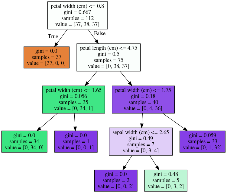![:scale 70%](images/instability_2.png)
]]
???
Another weakness of trees that I want to mention is that
they are very unstable. Using the iris dataset, let's say I
want a small tree. So I say I want a maximum of six leaves
nodes and I split my Iris dataset, and I build the tree, and
then I split the same data set again, and take a different
random state. Hopefully, I would assume that if it's the
same dataset, and I split randomly, then the models should
be similar. However, if you look at these models, even in
the root note, the very first decision it made is different.
One compares petal length to 2.45 while the other compares
pedal width to 0.8.

And the number of points that are split off are different
too. So there's not really an easy correspondence between
these two trees. So this is sort of a caveat about
interoperability. You can interpret the tree but maybe if
the dataset was only slightly different, the tree might look
completely different. So this tree structure is really
something that's very unstable.

---

# Feature importance

![:scale 80%](images/tree_importances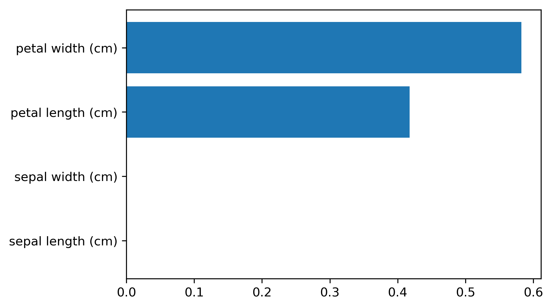.png)

]

???
Another interesting feature of trees that I want to mention
is feature importance. While looking at the trees, a nice
way to inspect the tree if it's small, if your trees very
big, it's very hard to understand what's happening in the
tree. So what you can get out is how important each feature
is for the tree. This is similar to the coefficients in the
linear model, where you can see that “this feature
influences the model in this way”. And the way this is done
is basically each time a particular feature was chosen in a
tree, you accumulate how much it decreased the impurity.
It'll give more importance to features that were used often
and where to use of it, than decreased impurity.

Problem with the importance is you have the same issues with
instability. Because the tree structures unstable, the
features picked is unstable and so the importance will be
unstable.

Similar to L1 norm, if you have too many correlated
features, it might pick one or the other. If you have very
correlated features, basically, the feature importance could
be anything. Any linear combination of the two is completely
equivalent. So keep that in mind when looking at feature
importance. But they’re a very nice way to summarize what
the tree does if you're in reasonably low dimensions and
your tree is big. Obviously, if you're in super high
dimensions, you might not be able to look at them, you might
be able to look at the most important features.

The question was if use a feature multiple times, do I add
up the degrees in purities and the answer is yes.

Question is can I explain the difference between
extrapolating and generalizing. In generalizing, usually you
make this IID assumption that you draw data from the same
distribution, and you have some samples from the
distribution from which you learn, and other samples from a
distribution which you want to predict. And if you're able
to predict well, then it is generalizing.

Here in the extrapolation example, the distribution that I
want to try to predict on was actually different from the
distribution I learned on because they’re completely
disjoint. The years I trained on and the years that I'm
testing on are completely disjoint and the target range is
also completely disjoint. So this is not an IID task.

In particular, even if it was IID, extrapolation sort of
means looking at things outside the training set.

One more comment about feature importance is that they give
you the importance of a feature, but not the direction. If
you look at the linear model and you say that a coefficient
is large, or a coefficient is very small, this means for
regression, if it's larger than it has a positive influence
on target, or if it's classification, this feature has a
positive influence to being a member of this class. For
trees, you don't have the directionality, here you only get
this is important only to make a decision. And the
relationship with the class might not be monotonous.

So you only have a magnitude you don't have a direction in
the importance.

- Unstable Tree $\rightarrow$ Unstable feature importances.
- Might take one or multiple from a group of correlated features.
---

# Categorical Data

- Can split on categorical data directly
- Intuitive way to split: split in two subsets
- 2 ^ n_values many possibilities
- Possible to do in O(n_values . log(n_values)) exactly for gini index and binary classification.
- Heuristics done in practice for multi-class.
- Not in sklearn yet

???
You can use categorical data in trees, and you can do this
in R up to a couple of hundred different values. In
scikit-learns, unfortunately, it’s not there yet.

The cool thing about it working with categorical data is
that it allows you to split into any subsets of the
categories. So if you have, let's say have one categorical
variable with five levels, or five different values, you
could split it in a tree in all possible ways. So in three,
two, four, one and with all of the possible combinations.

Usually, if you would want to do that you will need to try
out two to the power number of values many possibilities for
the splits, two to the power five in this example. That
might not be feasible. But actually, for some criteria, for
example, for Gini index you can do this efficiently in
linear time.

So in scikit-learn right now, you have to use one hot
encoding, which is not powerful because one hot encoding can
only split one feature at a time. So you would need to grow
a much deeper tree to split categorical variable in all
possible ways.

There's also I think in R there's a bunch of tree
implementations that work with missing values and there are
several different strategies to deal with missing values.

But it's also not entirely clear which strategy to deal with
a missing value in trees is the best. So one strategy is, if
you have a missing value, you can basically go down both
sides at once, if the question is about the value that's
missing, just go down both things. But that's kind of slow.
The other thing that it's actually just another value you
can split on and you can say, “if I split on a missing
value, I have a separate branch just for missing values.”

But you can easily emulate this by replacing it with a
binary feature which says missing or not missing.

---
class:spacious
# Predicting probabilities
- Fraction of class in leaf.
- Without pruning: Always 100% certain!
- Even with pruning might be too certain.
???
You can also predict probabilities with trees. Although, I
would recommend against it. The issue with trees is that
they are very good at overfitting, they can fit anything if
I grow them deep enough. If I grow them to the full depth,
they will always be 100% certain. Because the probability is
the fraction of the number of points in the leaves that
belong to this class. So if I have a leaf with like 10 data
points, and 7 of them belong to class A, then it will say,
with 70% probability a point here is class A. But if you
split until everything's pure, it will always be 100%
certain, which is pretty meaningless.

So you can do some pruning, and you can restrict the rows of
the tree, but it still might be certain, and so the
probability estimates that come out of a tree might not be
very good.

FIXME PLOT
---

# Random Forests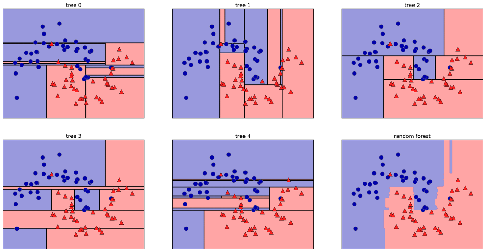

???
Here example of a random forest on a 2-dimensional dataset.
- Smarter bagging for trees!
---

# Randomize in two ways

- For each split:
  - Pick random sample of features

- More trees are always better
]

![:scale 100%](images/bootstrap_sample.png)

![:scale 100%](images/feature_sample.png)
]

???
The way that random forest work is they randomize tree
building in two ways. As with bagging if you do a bootstrap
sample of the dataset, so each tree you take a bootstrap
sample of the data set and then for each split in the tree,
you take a sampling without replacement of the features. So
let's say you have this representation of the dataset again.
And for each node where you want to make a splitting
decision before you want to scan all over the features and
all the thresholds, you select just the subset of the number
of features and just look for splits there. And this is done
for each node independently. In the end, the tree will use
all the features probably, if it's deep enough, eventually
it might use all the features but you randomize the tree
building process in a way that hopefully de-correlated the
error of the different trees. And so this adds another
hyperparameter in the tree building.
---
class:some-space
# Tuning Random Forests

- Main parameter: max_features
  - around sqrt(n_features) for classification
  - Around n_features for regression

- n_estimators > 100
- Prepruning might help, definitely helps with model size!
- max_depth, max_leaf_nodes, min_samples_split again

???
Which are max features, which is the number of features that
you want to look at each split. So the heuristic is usually
for classification you want something like the square root
of the number of features, whereas, for regression, you
usually want something that is around the same size as the
number of features. This basically, controls the variance of
the model because if you set this to number of features, it
will be just sort of the old decision tree. If you set this
to one, it will pick a feature at random, and then it needs
to split on that feature, basically.

So this will be like a very, very random tree that probably
would grow very deep because it can really make good
decisions.

This is the main parameter that you need to tune, although
random forest is actually very robust to these parameter
settings. Usually, if you leave this to the default, it will
be reasonably well.

By default, in scikit-learn, the number of trees in the
forest is way too low. Usually, you want something like 100,
or 500 but scikit-learn only gives you like 10.

Sometimes people find that pre-pruning techniques like
maximum depth or maximum leaf nodes help. Generally, the
idea doesn't really matter that much, how good the vigil
trees are as long as you have enough of them. But limiting
the size of the tree will definitely help with model size.
That said, if you randomize a lot, these trees will grow
very deep. Because if you're unlucky, you'll always just
split on bad feature so you will always not really get much
further in getting pure leaves and so you need to do a lot
of splits. So setting something like max depth will allow
you to decrease RAM size and decrease prediction time.

---

# Variable Importance

.smaller[
```python
X_train, X_test, y_train, y_test = train_test_split(
    iris.data, iris.target, stratify=iris.target, random_state=1)
rf = RandomForestClassifier().fit(X_train, y_train)
rf.feature_importances_
plt.barh(range(4), rf.feature_importances_)
plt.yticks(range(4), iris.feature_names);
```
```array([ 0.126,  0.033,  0.445,  0.396])```
]
.center[
![:scale 40%](images/forest_importances.png)
]
???
As for the trees, for the random forest, I can get variable
importance. And these are more useful now because they're
more robust. Again, they don't have directionality.

But now, if you have two correlated features, probably if
you build enough trees, and because of the way they’re
randomized, both of these features will be picked some of
the time. And so if you average over all of the trees, then
both will have the same amount of importance. So this will
basically just give you like a smoother estimate of the
feature importance that will be more robust and will not
fail on correlated features.

---
class: center, middle

# Notebook: Trees