class: center, middle  ### Advanced Machine Learning with scikit-learn Part I/II # Model Evaluation in Classification Andreas C. Müller Columbia University, scikit-learn .smaller[https://github.com/amueller/ml-workshop-3-of-4] ??? FIXME macro vs weighted average example FIXME balanced accuracy? FIXME move mape before plotting? or all metrics after? FIXME remove regression, go into more depth on cost-sensitive! FIXME relate to calibration! move using metrics in CV to the end? How to pick thresholds in multi-class? --- class: centre,middle # Metrics for Binary Classification ??? --- # Review : confusion matrix .center[  ] .larger[ $$\text{Accuracy} = \frac{\text{TP} + \text{TN}}{\text{TP} + \text{TN} + \text{FP} + \text{FN}}$$ ] ??? Diagonal divided by everything. --- class: center, middle # Positive & Negative are arbitrary ## Though often the minority class is considered positive --- # .smaller[ ```python from sklearn.metrics import confusion_matrix, plot_confusion_matrix data = load_breast_cancer() X_train, X_test, y_train, y_test = train_test_split( data.data, data.target, stratify=data.target, random_state=0) lr = LogisticRegression().fit(X_train, y_train) y_pred = lr.predict(X_test) print(confusion_matrix(y_test, y_pred)) print(lr.score(X_test, y_test)) plot_confusion_matrix(lr, X_test, y_test, cmap='gray_r') ``` ``` [[48 5] [ 4 86]] 0.94 ``` ]  ??? confusion_matrix and accuracy_score take y_true, y_pred Note that plot_confusion_matrix takes the estimator. We might change that. We'll talk a bit more about that interface later. --- # Problems with Accuracy Data with 90% negatives: .smaller[ ```python from sklearn.metrics import accuracy_score for y_pred in [y_pred_1, y_pred_2, y_pred_3]: print(accuracy_score(y_true, y_pred)) ``` ``` 0.9 0.9 0.9 ``` ] -- .center[  ] ??? - Imbalanced classes lead to hard-to-interpret accuracy. --- class:split-40 # Precision, Recall, f-score .left-column[ `$$ \large\text{Precision} = \frac{\text{TP}}{\text{TP}+\text{FP}}$$`<br /> `$$\large\text{Recall} = \frac{\text{TP}}{\text{TP}+\text{FN}}$$`<br /> `$$\large\text{F} = 2 \frac{\text{precision} \cdot\text{recall}}{\text{precision}+\text{recall}}$$`] .right-column[ <br /> Positive Predicted Value (PPV) <br /> <br /> <br /> <br /> Sensitivity, coverage, true positive rate. <br /> <br /> <br /> <br /> Harmonic mean of precision and recall ] ??? All depend on definition of positive and negative. --- class: center, spacious # The Zoo  https://en.wikipedia.org/wiki/Precision_and_recall ??? --- class: compact # Normalizing the confusion matrix .smallest[ ```python confusion_matrix(y_true, y_pred) ```  ] .left-column[ .smallest[ ```python confusion_matrix(y_true, y_pred, normalize='true') ```  ] ] .right-column[ .smallest[ ```python confusion_matrix(y_true, y_pred, normalize='pred') ``` 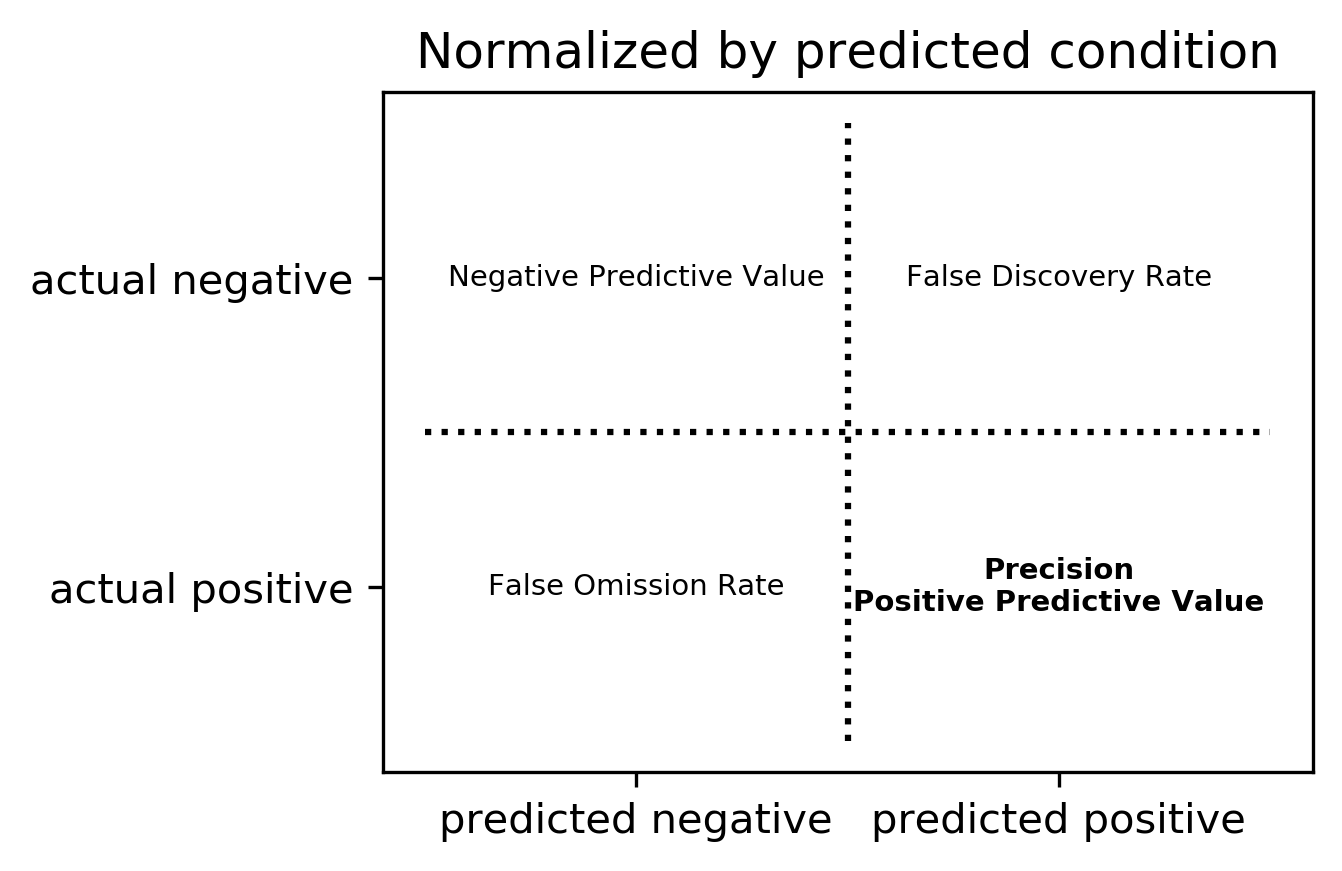 ] ] --- class:compact .smallest[ ```python classification_report(y_true, y_pred) ``` ] .left-column[ 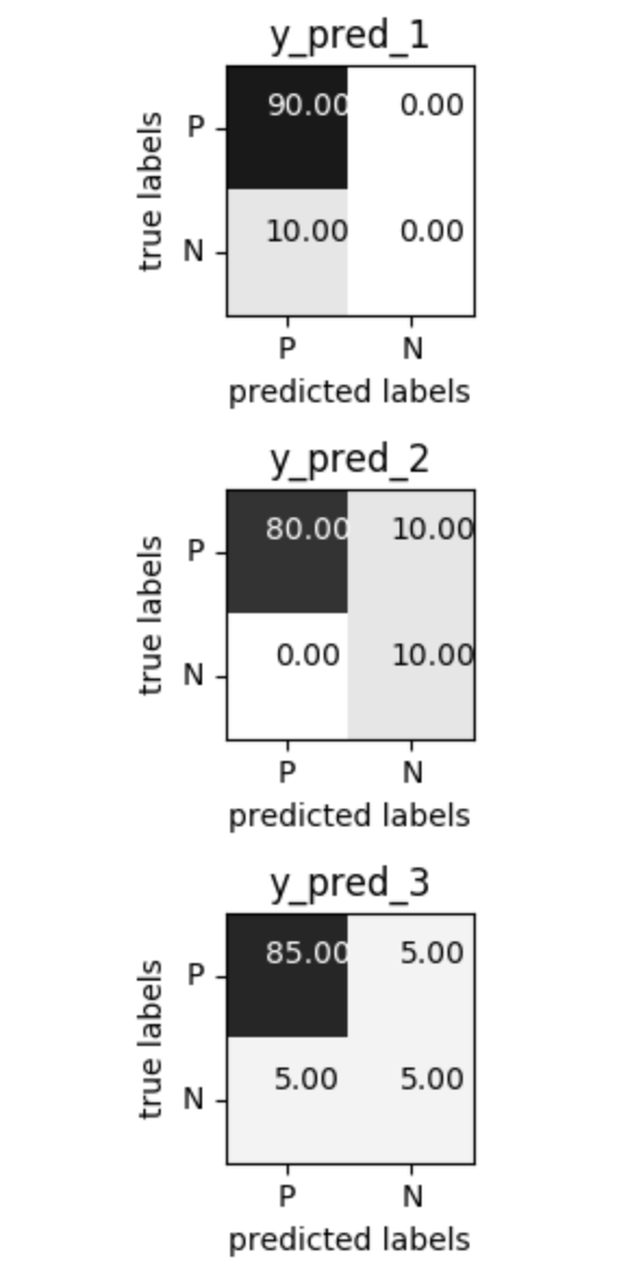] .smallest[ .right-column[ ``` precision recall f1-score support 0 0.90 1.00 0.95 90 1 0.00 0.00 0.00 10 accuracy 0.90 100 macro avg 0.45 0.50 0.47 100 weighted avg 0.81 0.90 0.85 100 precision recall f1-score support 0 1.00 0.89 0.94 90 1 0.50 1.00 0.67 10 accuracy 0.90 100 macro avg 0.75 0.94 0.80 100 weighted avg 0.95 0.90 0.91 100 precision recall f1-score support 0 0.94 0.94 0.94 90 1 0.50 0.50 0.50 10 accuracy 0.90 100 macro avg 0.72 0.72 0.72 100 weighted avg 0.90 0.90 0.90 100 ``` ]] ??? --- # Averaging strategies `$$\text{macro }\frac{1}{\left|L\right|} \sum_{l \in L} R(y_l, \hat{y}_l)$$` `$$\text{weighted } \frac{1}{n} \sum_{l \in L} n_l R(y_l, \hat{y}_l)$$` .smaller[ ```python print("Weighted average: ", recall_score(y_test, y_pred_1, average="weighted")) print("Macro average: ", recall_score(y_test, y_pred_1, average="macro")) ``` ``` Weighted average: 0.90 Macro average: 0.50 ``` ] <br /> ??? Two common ways to approach multitask is to look at averages over binary metrics. So you can do binary metrics for recall, precision f1 score. But in principle, you could do it for more things. And in scikit-learn has several averaging strategies. There is macro, weighted, micro and samples. You should really not worried about micro samples, which only apply to multi-label prediction. We haven't talked about multi-label prediction and we're not going to talk about multi-label prediction. Multi-level prediction is when each sample can have multiple labels. Macro and weighted are the two options. They are interesting. For example, for recall, we can look at macro average recall, which is the average over all the labels and then the recall for just this label. So basically, here y_l is the true label, y ̂ is the predicted label. The positive class is now label l, and the negative classes is any other label, so this is sort of one versus rest version of recall. You can also do a weighted average, you weight by the number of samples in each class, and then divide by the total number of samples. So again, for each class, I compute recall for that class, and then I weight that by the number of samples. This is actually what classification report reports here. It's kind of interesting that if you do this, then actually looking at precision or recall just by themselves is informative. So if you look at macro average recall, that's actually also called balanced accuracy or if you look at macro average precision, this will be the useful metric by itself, because it looks at the precision of each of the classes. So basically, the choice between macro and weighted is whether you think each class should have the same weight, or each sample should have the same weight. Let’s say, we have recall for one class is 1 and for the other class 0. And for the majority class recall is 1 and for the minority, class recall is 0. For macro average recall, you would get 0.5 because you just take the average of the two. If you look at a weighted, then the outcome would be the proportion of the positive class. So if 90% of the data is positive, you will get 90% here. So basically weighted takes the class sizes into account and so the bigger classes count for more. If you're actually interested in the smaller classes, macro is probably better because each class weights the same. Which one is the best really depends on your application? Macro is counted each class the same while weighted is count each sample the same. I did this here on the digit data set, which is basically balanced and so there's no difference. micro vs macro same for other metrics. --- class: spacious # Balanced Accuracy .smaller[ ```python balanced_accuracy_score(y_t, y_p) == recall_score(y_t, y_p, average='macro') ``` ] $$\text{balanced_accuracy} = \frac{1}{2}\left( \frac{TP}{TP + FN} + \frac{TN}{TN + FP}\right )$$ - Always 0.5 for chance predictions - Equal to accuracy for balanced datasets --- # Mammography Data .smallest[ .left-column[ ```python from sklearn.datasets import fetch_openml # mammography https://www.openml.org/d/310 data = fetch_openml('mammography', as_frame=True) X, y = data.data, data.target X.shape ``` (11183, 6) ```python y.value_counts() ``` ``` -1 10923 1 260 ``` ] .right-column[ .center[ 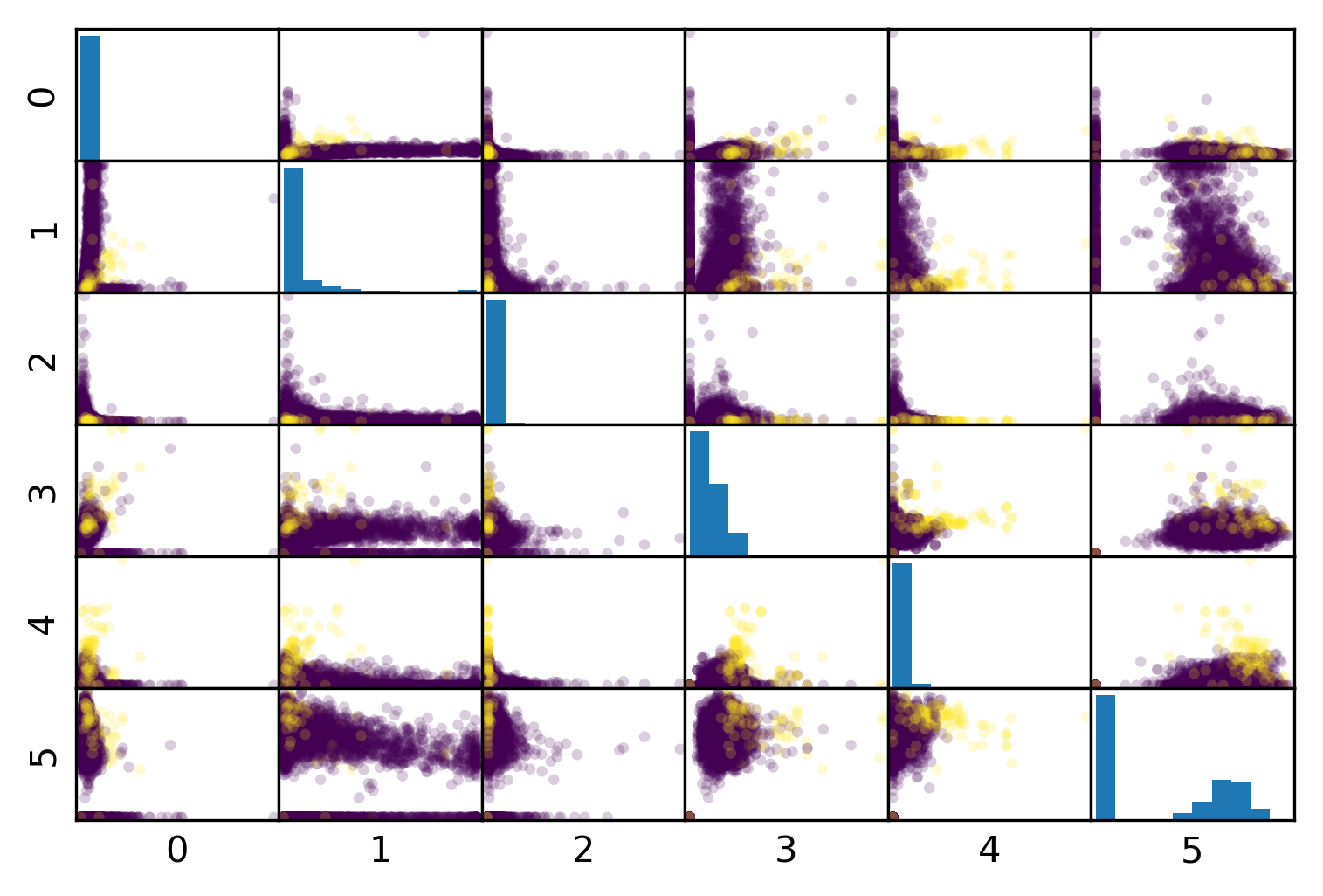 ] ] .reset-column[ ```python # make y boolean # this allows sklearn to determine the positive class more easily X_train, X_test, y_train, y_test = train_test_split(X, y == '1', random_state=0) ``` ] ] ??? I use this mammography data set, which is very imbalanced. This is a data set that has many samples, only six features and it's very imbalanced. The datasets are about mammography data, and whether there are calcium deposits in the breast. They are often mistaken for cancer, which is why it's good to detect them. Since its rigidly low dimensional, we can do a scatter plot. And we can see that these are much skewed distributions and there's really a lot more of one class than the other. --- .smallest[ .left-column[ ```python svc = make_pipeline(StandardScaler(), SVC(C=100, gamma=0.1)) svc.fit(X_train, y_train) svc.score(X_test, y_test) ``` ``` 0.986 ``` ] .right-column[ ```python rf = RandomForestClassifier() rf.fit(X_train, y_train) rf.score(X_test, y_test) ``` ``` 0.989 ``` ] ] -- .reset-column[ ] .smallest[ .left-column[ ``` precision recall f1-score support False 0.99 1.00 0.99 2732 True 0.81 0.53 0.64 64 accuracy 0.99 2796 macro avg 0.90 0.76 0.82 2796 weighted avg 0.98 0.99 0.99 2796 ``` ] .right-column[ ``` precision recall f1-score support False 0.99 1.00 0.99 2732 True 0.90 0.56 0.69 64 accuracy 0.99 2796 macro avg 0.94 0.78 0.84 2796 weighted avg 0.99 0.99 0.99 2796 ``` ] ] --- class:spacious # Goal setting! - What do I want? What do I care about? - Can I assign costs to the confusion matrix? - What guarantees do we want to give? ??? (precision, recall, or something else) (i.e. a false positive costs me 10 dollars; a false negative, 100 dollars) --- # Changing Thresholds .tiny-code[ ```python y_pred = rf.predict(X_test) print(classification_report(y_test, y_pred)) ``` ``` precision recall f1-score support False 0.99 1.00 0.99 2732 True 0.90 0.56 0.69 64 accuracy 0.99 2796 macro avg 0.94 0.78 0.84 2796 weighted avg 0.99 0.99 0.99 2796 ``` ```python y_pred = rf.predict_proba(X_test)[:, 1] > .30 print(classification_report(y_test, y_pred)) ``` ``` precision recall f1-score support False 0.99 0.99 0.99 2732 True 0.71 0.64 0.67 64 accuracy 0.99 2796 macro avg 0.85 0.82 0.83 2796 weighted avg 0.99 0.99 0.99 2796 ``` ] ??? --- class: compact # Precision-Recall curve .smaller[ ```python svc = make_pipeline(StandardScaler(), SVC(C=100, gamma=0.1)) svc.fit(X_train, y_train) plot_precision_recall_curve(svc, X_test, y_test, name='SVC') ``` ] .center[ 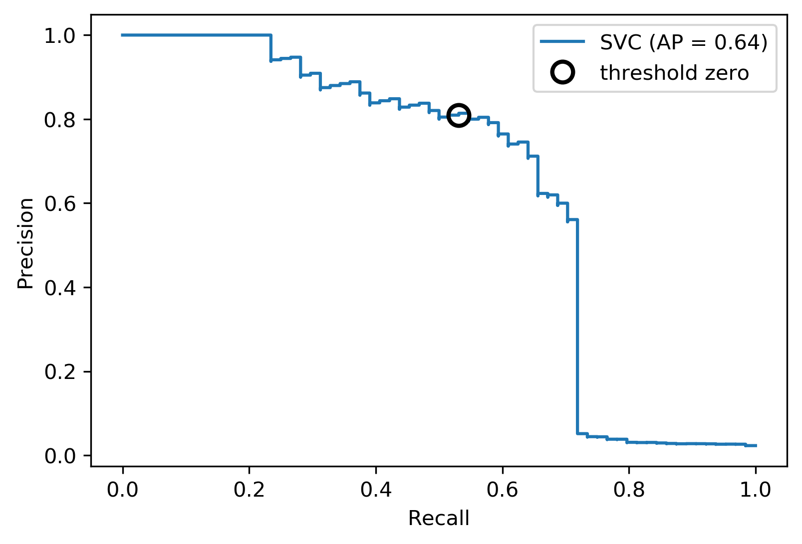 ] ??? --- # Side note: Scikit-learn plotting API .smaller[ ```python prc = plot_precision_recall_curve(svc, X_test, y_test, name='SVC') # plot pops up here prc ``` ``` <sklearn.metrics._plot.precision_recall_curve.PrecisionRecallDisplay at ...> ``` ```python vars(pr_svc) ``` ``` {'precision': array([0.023, 0.023, 0.023, ..., 1. , 1. , 1. ]), 'recall': array([1. , 0.984, 0.984, ..., 0.031, 0.016, 0. ]), 'average_precision': 0.6743452407177641, 'estimator_name': 'Pipeline', 'line_': <matplotlib.lines.Line2D at ... >, 'ax_': <matplotlib.axes._subplots.AxesSubplot at ...>, 'figure_': <Figure size 432x288 with 1 Axes>} ``` ```python # plot again without recomputing prc.plot() ``` ] --- class: compact # ROC Curve .center[ ## (Receiver Operating Characteristic) ] .smaller[ ```python plot_roc_curve(svc, X_test, y_test, name='SVC') ``` ] .center[  ] ??? --- .left-column[ # PR-Curve  ] .right-column[ # ROC-Curve  ] .reset-column[ - Share one axis (though transposed!?) - Interpolation is meaningful on ROC curve but not PR curve ] --- # Comparing RF and SVC .smallest[ ```python pr_svc = plot_precision_recall_curve(svc, X_test, y_test, name='SVC') # if we used computed before, we could just call pr_svc.plot() # using ax=plt.gca() will plot into the existing axes instead of creating new ones pr_rf = plot_precision_recall_curve(rf, X_test, y_test, ax=plt.gca()) ``` ] .center[  ] ??? We’re going to compare random forest and support vector machine. You can see they're sort of similar. But in some areas, they are different. For example, you can see that the random forest is little bit more stable for very high precision but in some places the SVM is better than random forest and vice versa. So which of the two is better classifier really depends on which area you're interested in. By comparing these two curves, again, sort of a very fine grain thing that you can do manually, if you want to do this for many models, and want to pick the best model. This is maybe not really feasible. So you might want to summarize this in a single number. So one number you could think of is, while I know I definitely want to have a recall of 90% so I'm going to put my threshold here and compare at that threshold. If you don't really have a particular goal yet, you can also consider all thresholds at once, and basically compute the area under this curve. It's not exactly the same but that's sort of what average precision does. --- # Average Precision .center[  ] ??? Average precision basically does a step function integral of this thing. So for each possible threshold, you look at the precision at this threshold times the change in recall. So this is like fitting a step function under the curve and then computing the integral. This allows you to basically take all possible thresholds into account at once. Q: How do I adjust the precision-recall ratio for the random forest? I mean, it says predict_proba. So I can alter threshold that at different values if I want. For a support vector machine, which doesn't have predict_proba, I can also adjust the threshold the decision function. Average precision is a pretty good metric to basically compare models if there are imbalanced classes. Related to area under the precision-recall curve (with step interpolation) --- # Area Under ROC Curve (aka AUC) .center[  ] - Always .5 for random/constant prediction ??? And so when you look at the area under the curve, which is called ROC AUC, it's always 0.5 for random or constant predictions. So it's very easy to say, how much better than random are you if you look at ROC AUC. I encourage you to read the paper in the link. One thing is that the ROC curve is usually much smoother and it makes more sense to interpolate it, where the precision-recall curve makes less sense to interpolate us. But the precision-recall curve can sometimes pick up on more fine-grained differences. Even though AUC stands for area under the curve, if you see it in literature always means the area under the receiver operating curve. So AUC always means ROC AUC. AUC is a ranking metric. So it takes all possible thresholds into account, which means that it's independent of the default thresholds. So again, you can have something with very low accuracy but still with perfect ROC AUC. --- # Keep in mind: ranking vs predictions ```python dec = svc.decision_function(X_test) np.all((dec > 0) == svc.predict(X_test)) ``` ``` True ``` ```python print(f1_score(y_test, dec > 0)) print(average_precision_score(y_test, dec)) ``` ``` 0.641 0.635 ``` -- ```python dec_new = dec - 10 print(f1_score(y_test, dec_new > 0)) print(average_precision_score(y_test, dec_new)) ``` ``` 0.0 0.635 ``` --- # Threshold and ranking metrics .left-column[ .tiny[ ```python from sklearn.metrics import f1_score f1_rf = f1_score(y_test, rf.predict(X_test)) print(f"f1_score of random forest: {f1_rf:.3f}") f1_svc = f1_score(y_test, svc.predict(X_test)) print(f"f1_score of svc: {f1_svc:.3f}") ``` ``` f1_score of random forest: 0.709 f1_score of svc: 0.715 ``` ```python from sklearn.metrics import balanced_accuracy_score ba_rf = balanced_accuracy_score(y_test, rf.predict(X_test)) print(f"Balanced accuracy of random forest: {ba_rf:.3f}") ba_svc = balanced_accuracy_score(y_test, svc.predict(X_test)) print(f"Balanced accuracy of svc: {ba_svc:.3f}") ``` ``` Balanced accuracy of random forest: 0.765 Balanced accuracy of svc: 0.764 ``` ] ] .right-column[ .tiny[ ```python from sklearn.metrics import average_precision_score ap_rf = average_precision_score( y_test, rf.predict_proba(X_test)[:, 1]) print(f"Average precision of random forest: {ap_rf:.3f}") ap_svc = average_precision_score( y_test, svc.decision_function(X_test)) print(f"Average precision of svc: {ap_svc:.3f}") ``` ``` Average precision of random forest: 0.682 Average precision of svc: 0.693 ``` ```python from sklearn.metrics import roc_auc_score auc_rf = roc_auc_score(y_test, rf.predict_proba(X_test)[:, 1]) print(f"Area under ROC curve of random forest: {auc_rf:.3f}") auc_svc = roc_auc_score(y_test, svc.decision_function(X_test)) print(f"Area under ROC curve of svc: {auc_svc:.3f}") ``` ``` Area under ROC curve of random forest: 0.936 Area under ROC curve of svc: 0.817 ``` ]] ??? Previously, I just have sort of a simple comparison between f1 and average precision. I'm comparing these two models. So if I look at f1 score, it's going to compare basically these two points and the SVC is slightly is better. But F1 score only looks at the default threshold. If I want to look at the whole RC curve, I can use average precision. Even if I look at all possible thresholds, SVC is still better. Average precision is sort of a very sensitive metric that allows you to basically make good decisions even if the classes are very imbalanced and that also takes all possible thresholds into account. One thing that you should keep in mind if you use this is that this does not give you a particular threshold. For example, if you use the default threshold, your accuracy might be zero. This only looks at ranking. The curve and the area under the curve, don't depend on where the default threshold is. So if you predict everything, like for some weird reason, if you predict everything as the minority class, your accuracy will be really bad. But if they are ranked in the right order, so that all the positive classes are ranked higher than the negative classes, then you might still get an area under the curve that's very close to one. So this only looks at ranking. AP only considers ranking! --- # Summary of metrics for binary classification Threshold-based: - (balanced) accuracy - precision, recall, f1 Ranking: - average precision - ROC AUC ??? So let's briefly summarize the metrics for binary classification. So there are basically two approaches. One looks just at the predictions or look at soft predictions and take multiple thresholds into account. So the ones that I called threshold base, which is for single threshold, the ones that we talked about in our accuracy, which is just a fraction of correctly predicted, precision, recall, and f1. So the issue with accuracy is obviously that it can't distinguish between things that are quite different, for example, for imbalanced data sets, the classifier always predicts majority class often has like very high accuracy but tells you nothing. So in particular, for imbalanced classes, accuracy is a pretty bad measure. Precision and recall together are pretty good measures, though you always need to look at both numbers. One way to look at both numbers at once is the f1 score, though, using the harmonic mean is a little bit arbitrary. But still, only f1 score is a somewhat reasonable score if you only look at the actual predicted classes. For the ranking based losses, I think both average precision and ROC AUC are pretty good choices, ROC AUC, I like it because I know what 0.5 means, while for average precision, it's a little bit more tricky to see what the different orders of magnitude mean, or the different scales mean, but it can be more fine-grained measure. And so if you want to do cross-validation, my go-to is usually ROC AUC. In particular, for imbalance binary datasets, I would usually use ROC AUC. But then make sure that your threshold is sensible, but anything other than accuracy is okay. Just don’t look at only precision or only recall, if you do a grid search for just precision, you will probably get garbage results. add log loss? --- class: centre,middle # Multi-class classification ??? The next thing I want to talk about is multiclass classification. --- class:split-40 #Confusion Matrix .left-column[ .tiny-code[ ```python from sklearn.datasets import load_digits from sklearn.metrics import accuracy_score digits = load_digits() # data is between 0 and 16 X_train, X_test, y_train, y_test = train_test_split( digits.data / 16., digits.target, random_state=0) lr = LogisticRegression().fit(X_train, y_train) pred = lr.predict(X_test) print("Accuracy: {:.3f}".format(accuracy_score(y_test, pred))) plot_confusion_matrix(lr, X_test, y_test, cmap='gray_r') ``` ``` Accuracy: 0.964 ``` 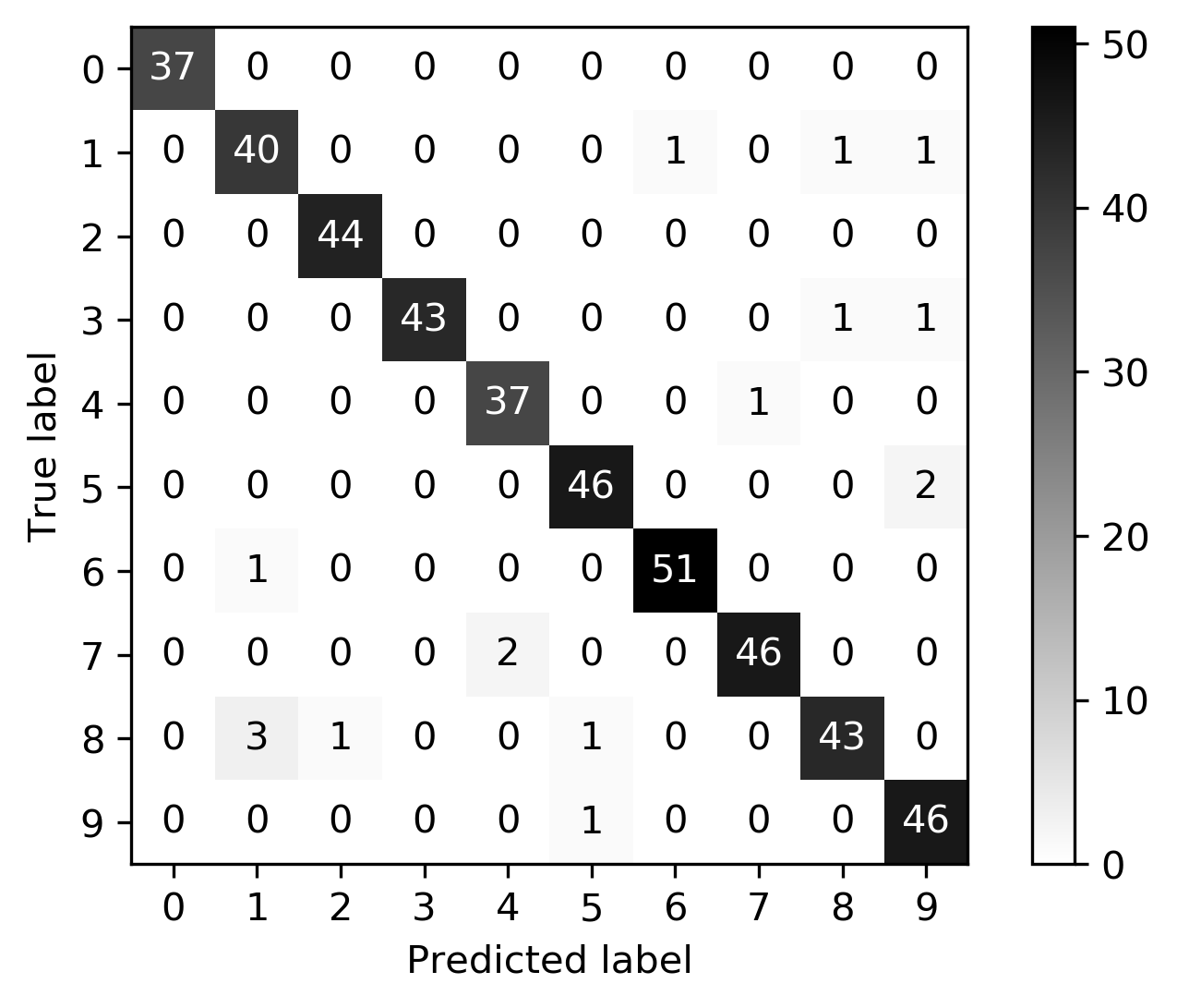 ] ] .right-column[ .tiny-code[ ```python print(classification_report(y_test, pred)) ``` ``` precision recall f1-score support 0 1.00 1.00 1.00 37 1 0.91 0.93 0.92 43 2 0.98 1.00 0.99 44 3 1.00 0.96 0.98 45 4 0.95 0.97 0.96 38 5 0.96 0.96 0.96 48 6 0.98 0.98 0.98 52 7 0.98 0.96 0.97 48 8 0.96 0.90 0.92 48 9 0.92 0.98 0.95 47 accuracy 0.96 450 macro avg 0.96 0.96 0.96 450 weighted avg 0.96 0.96 0.96 450 ``` ] ] ??? So again, for multiclass classification, you look at the confusion matrix. It's even more telling in a way than it was for binary classification but it's also pretty big. So here, I'm using the digital data set, which has 10 classes, and here's the confusion matrix. The diagonal is everything that's correct, the off-diagonal are mistakes. And you can see very fine-grained which classes were mistaken for which other classes. So this is very nice if you want to look in a very detailed view of the performance of the classifier. But again, you can't really use it for model selection, or not easily. You can also again, look at the classification report, which will give you precision-recall and F score for each for the classes, again, very, very fine grained. So you can see, for example, that Class 0, was predicted while Class 8 is the hardest. It might make more sense to look at in precision average classes, recall over the classes or f1 score for the classes. --- # Multi-class ROC AUC - Hand & Till, 2001, one vs one `$$ \frac{1}{c(c-1)}\sum_{j=1}^{c}\sum_{k \neq j}^{c} AUC(j,k)$$` - Provost & Domingo, 2000, one vs rest `$$ \frac{1}{c}\sum_{j=1}^{c}p(j) AUC(j,\text{rest}_j)$$` ??? You can do that similar for ROC AUC. It will soon be available in scikit-learn. There are basically two versions of doing multiclass ROC AUC. One is called Hand & Till while the other is called Provost & Domingo. And the first one is basically one versus one where you iterate over all the classes, and then you iterate over all the other classes, then you look at the AUC of one class versus the other class. And this one is basically one versus rest where you look at the AUC of one class versus all the other classes. H&T is not weighted whereas, on P&D, p(j) means number of samples in j, and P&D is weighted. You can also do weighted OvO or unweighted OvR. There are at least 4 different ways to do multi-class AUC. It’s not clear to me how they behave in practice. If you weighted then you count the samples are the same weight. If you do unweight, you give the different classes the same weight. So this is definitely a pretty good metric if you want a ranking metric for multi-class classification. FIXME unify notation with slide on averaging --- # Summary of metrics for multiclass classification Threshold-based: - accuracy - precision, recall, f1 (macro average, weighted) Ranking: - OVR ROC AUC - OVO ROC AUC ??? The threshold based ones are sort of the same, only now looking at only precision, or only recall, if you average over all the classes actually makes sense. So you can do a grid search over macro average recall, and it'll give you reasonable results. For ranking, in theory, you could also do OvR or OvO on the precision-recall curve. But I haven’t seen anyone done that or any papers on that. So let's not do that for now. Both can be weighted or unweighted versions of that. Both are great for imbalance problems again, but now you have to pick multiple thresholds and it's unclear how to do that well or at least for me. So let’s say you use OVO ROC and you get a classifier with a high value there, and now you want to make predictions. What thresholds do you use? I don't actually have a good answer. Because you need n minus one different threshold to actually make a decision. So for this reason, probably for multi-class, I might not use the ranking metrics unless you have to be cursed, they're sort of hard to interpret. And I would probably use something like macro average precision or macro average recall or macro average f1. --- class: centre,middle # Metrics for regression models ??? --- class:spacious # Build-in standard metrics - $\text{R}^2$ : easy to understand scale - MSE : easy to relate to input - Mean absolute error, median absolute error: more robust ??? The built-in standard metrics by default in scikit-learn uses R squared. The other obvious metric is Mean Squared Error. The good thing about R squared is it's around zero and maximum of one. It's very easy to understand the scale. If it's close to one is good. If it's negative, it's really bad. If it's close to zero, it's bad. While the MSE is easier to relate to the input. So the scale of the mean squared error is sort of relates to the scale of the output. You can also use things like mean absolute error, and median absolute error, which is more robust. If you square things, then outliers have a very big impact. So if we don't square things, then outliers have less of an impact. So often people prefer to use mean absolute error to limit the impact of outliers. If being low is good, you need to have a neg before and if being high is good you won't be needing to it be neg. I think these are actually the only metrics that are in scikit-learn. --- class:spacious # Absolute vs Relative: MAPE `$$ \text{MAPE} = \frac{100}{n} \sum_{i=1}^{n}\left|\frac{y-\hat{y}}{y}\right|$$` .center[ 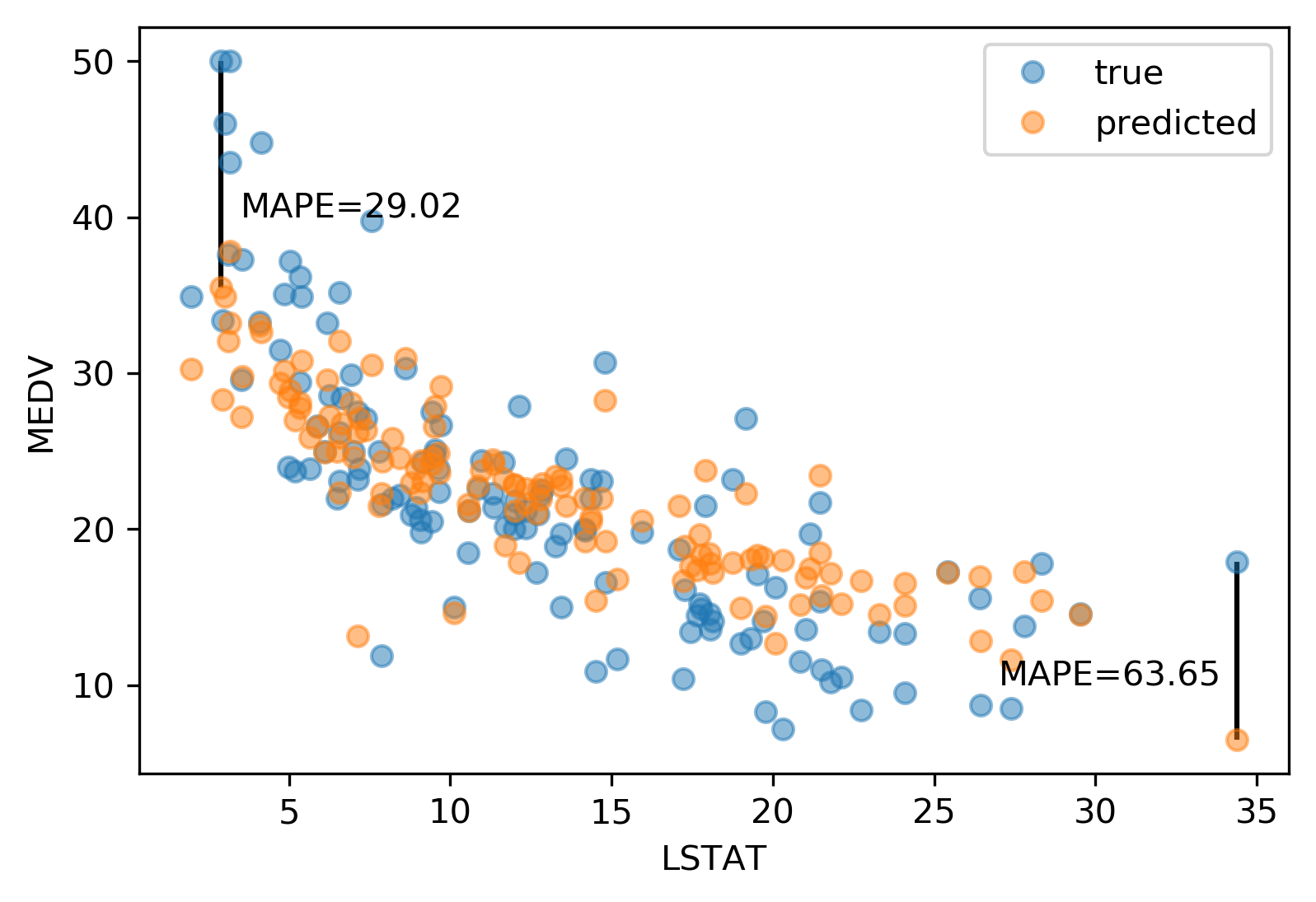 ] ??? There's another metric I want to talk about called MAPE. Which comes up in particular in forecasting. MAPE stands for Mean Absolute Percentage Error. MAPE captures is the percentage error. It divides the residual by the true value. Here for each individual data point, we’re dividing by the true value. Basically, what that means is that if a data point is large, we care less about how well we predict it. Basically, we allow larger error bars around high values. And I tried to plot this here, this is sort of for the one feature, LSTAT, to have like a reasonable x-axis since that helps us visualize this. And so here is the true dataset in blue and the predictive dataset in orange predicted using all features. And so in the bottom right, you can see it that we are under predicting by about 10. And this gives us a MAPE of 36%. On the top left, we are under predicting by even more, but the MAPE is smaller. So even though the absolute error on the top is bigger than the absolute error on the bottom, the relative error in the top is much smaller than the relative error in the bottom. This is a very commonly used measure in forecasting. Be careful when to use it because sometimes it might be not super intuitive. In particular, if something is not defined, if anything is zero, and if something is very close to zero, you need to perfectly predict it otherwise, you have unbound error. So this is usually used for things that are greater than one. --- class: spacious # Over vs under - Overprediction and underprediction can have different cost. - Try to create cost-matrix: how much does overprediction and underprediction cost? - Is it linear? ??? One of the things you might want to consider is looking at how much you under predict versus how much you over predict. In a business case under-predicting and overpredicting can have different costs. You can try to create a cost matrix to state the amount of underprediction or over prediction. You can also try to ask if this relationship linear. The most natural thing to do would be to look at the residuals and ask yourself how much it costs if I make a prediction that has this residual. And ask is it a linear function of the error or not. Though this only looks at the absolute error, you can also do the same for relative error. So maybe the first decision is, should I look at absolute errors, or should I look at the relative errors. And then for each particular bin of how much I'm over or under predicting, how much this costs me. --- # Prediction plots .wide-left-column[ .smaller[ ```python from sklearn.linear_model import Ridge from sklearn.datasets import load_boston boston = load_boston() X_train, X_test, y_train, y_test = train_test_split( boston.data, boston.target) ridge = Ridge(normalize=True) ridge.fit(X_train, y_train) pred = ridge.predict(X_test) plt.plot(pred, y_test, 'o') ``` ]] .narrow-right-column[ 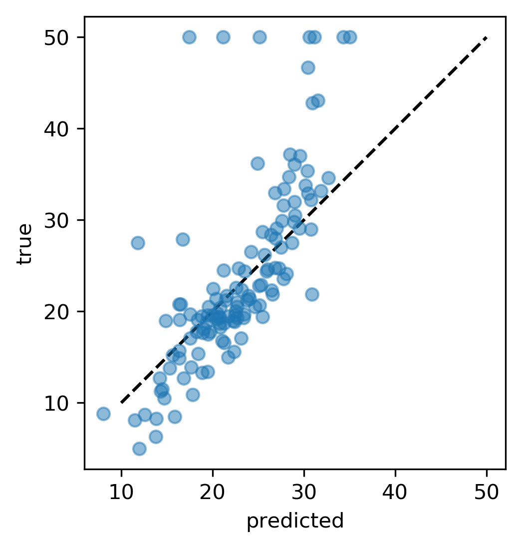 ] ??? I think one of the best debugging tools is prediction plots, where you plot the predicted versus the true outcome. This is on the Boston dataset here, I just do a ridge regression model. And so here, I plot the predicted outcome by the ridge regression on the test data set versus the true outcome. And so ideally, it should be the same, they it should be on the diagonal. But you can see that there's like, a couple things wrong with it. So for example, there are a couple of things where the true prediction is 50K, but I under predict severely. There’s a lot of underprediction going on. In particular, for low values, I’m predicting too high and for high values, I’m predicting too low. Looking at this you can see different trends and see if there are any trends or not. --- class:split-40 # Residual Plots .left-column[ <br /> 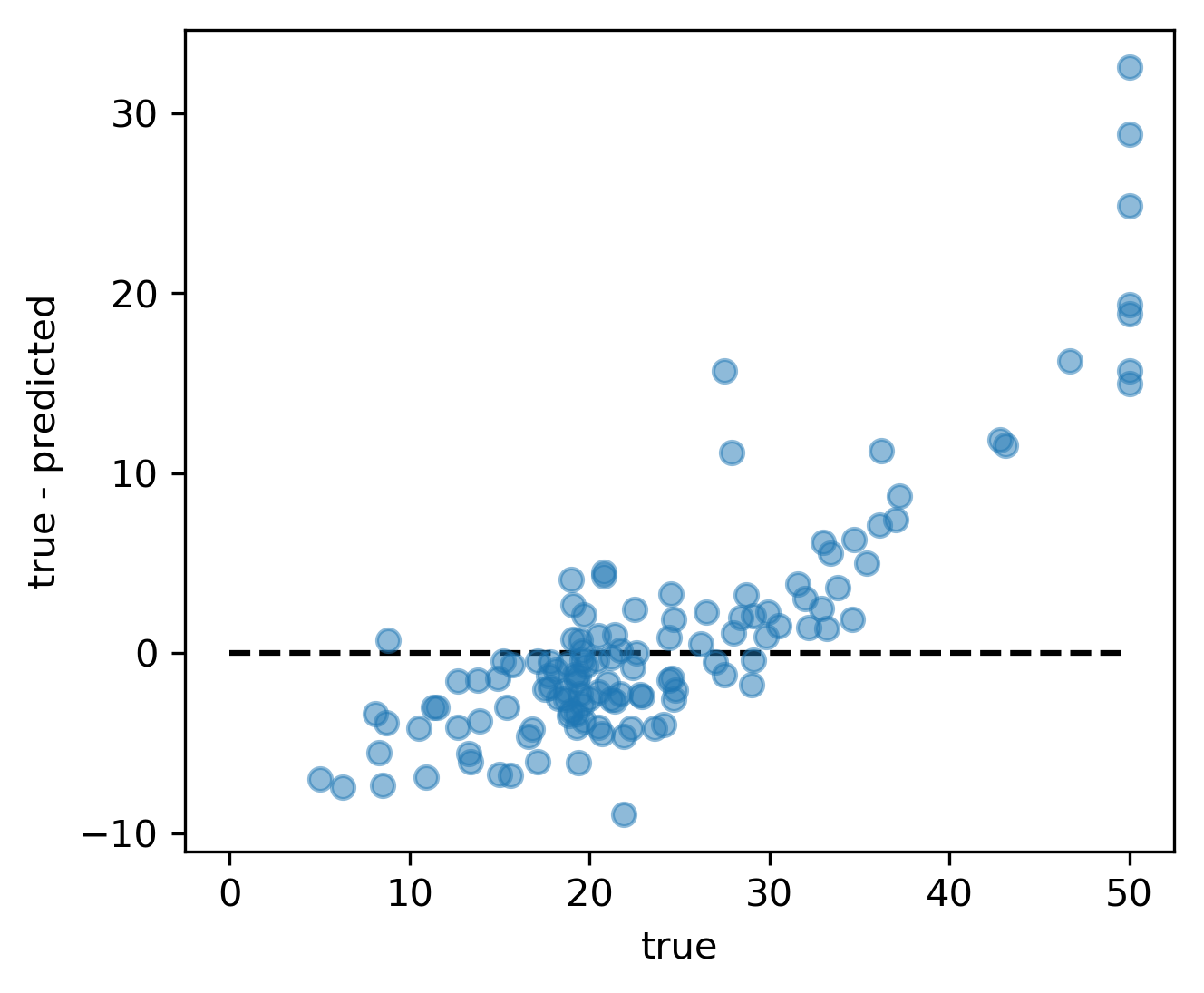] .right-column[ ] ??? A different way to look at this is to basically rotate that 45 degrees. So here we are looking at the true versus true minus predicted. This allows you even more easily to see if there are trends, and you can see that basically, we're over predicting for low values and we're under predicting for high values. You can also look at the histogram of the residuals and you can see that they’re mostly centered around zero, which is good so there's probably no systematic bias but you can see that there are some values where we underpredict by quite a lot. These are nice because you can do these plots no matter what dimension your data set is. --- # Target vs Feature  ??? If you want to look at in more detail, you can look at per feature plots. --- # Residual vs Feature  ??? Here, I'm plotting y test minus the prediction against each of the features and see if there are particular aspects of the feature that are not captured. For example, you can see here that for a low LSTAT, we are underpredicting more than for a high LSTAT. That shows that there might be trends in these features that we're not capturing. The X-axis is features. For each data point in the test dataset, I look at the value of this feature, and I look at the residual, which is the true value minus the prediction. Ideally, this should all be sort of horizontal because the errors that the model makes should be independent of all of the features. If the error that the model makes is not independent of the feature that means there's some aspect of the feature that the model didn't capture. This is basically the dependence of the target on the feature that is not captured by the prediction. And you can meditate that and then at some point it'll make sense. These are all more and more fine grain plots to understand the errors that you're making. --- # Picking metrics - Accuracy rarely what you want - Problems are rarely balanced - Find the right criterion for the task - OR pick a substitude, but at least think about it - Emphasis on recall or precision? - Which classes are the important ones? ??? In summary, for both multiclass and binary, you should really think about what your metrics are. And unless your problem is balanced, and even maybe then don't use accuracy. Accuracy is really bad. Problems are rarely balanced, in a real world and usually there heavily unbalanced unless someone artificially balances them. So it's really important to think about what is the right criterion for a particular task, and then you can optimize that criterion. So as I said, that can be like having costs associated with the confusion matrix, emphasizing precision or recall, setting specific goals such as have recall of at least X percent, or have precision of at least X percent and for multi-class deciding whether are all the classes the same importance, or all the samples the same importance, what are the important classes, even for binary, which one is the positive class? So whenever you talk about precision and recall, it’s important to think about which one is the positive class and how will changing the positive class change these two values? So and then finally, obviously, am I going to use the default threshold? Why am I going to use the default threshold? Do I use a ranking based metric? Or is there a reason why I would want to use a ranking based metric? --- # Using metrics in cross-validation .smaller[ ```python cancer = load_breast_cancer() X, y = cancer.data, cancer.target # default scoring for classification is accuracy rf = RandomForestClassifier(random_state=0) print("default scoring ", cross_val_score(rf, X, y)) # providing scoring="accuracy" doesn't change the results explicit_accuracy = cross_val_score(rf, X, y, scoring="accuracy") print("explicit accuracy scoring ", explicit_accuracy) ap = cross_val_score(rf, X, y, scoring="average_precision") print("average precision", ap) ``` ``` default scoring [0.93 0.947 0.991 0.974 0.973] explicit accuracy scoring [0.93 0.947 0.991 0.974 0.973] average precision [0.992 0.973 0.999 0.995 0.999] ``` ] ??? So once you pick them, it's very easy to use any of these metrics in scikit-learn. So they're all functions inside the metrics module, but usually, you're going to want to use them in for cross-validation, or grid search. And then it's even easier. There's argument called scoring. It takes a string or a callable. And so here, if you give it a string, it'll just do the right thing automatically. By default its accuracy. So if you don't do anything, it's the same as if you provide accuracy. But you can also set ROC AUC, and it's going to use ROC AUC. So the thing is ROC AUC actually needs probabilities right or a decision function, so behind the scenes, it does the right thing and gets out the decision function for the positive class to compute the ROC AUC correctly. Using better a metric than accuracy is as simple as saying scoring equal to something. And it’s exactly the same as in grid search CV. So if you want to do a grid search CV or randomized search CV, you can set scoring equal to ROC AUC or average precision or recall macro. Same for GridSearchCV <br /> Will make GridSearchCV.score use your metric! --- # Multiple Metrics ``` from sklearn.model_selection import cross_validate res = cross_validate(RandomForestClassifier(), X, y, scoring=["accuracy", "average_precision", "recall_macro"], return_train_score=True, cv=5) pd.DataFrame(res) ``` .tiny[ <table border="1" class="dataframe"> <thead> <tr style="text-align: right;"> <th></th><th>fit_time</th><th>score_time</th><th>test_accuracy</th><th>train_accuracy</th><th>test_average_precision</th><th>train_average_precision</th><th>test_recall_macro</th><th>train_recall_macro</th></tr> </thead> <tbody> <tr><th>0</th><td>0.171312</td><td>0.016973</td><td>0.921053</td><td>1.0</td><td>0.992115</td><td>1.0</td><td>0.918277</td><td>1.0</td></tr> <tr><th>1</th><td>0.133090</td><td>0.017563</td><td>0.938596</td><td>1.0</td><td>0.972293</td><td>1.0</td><td>0.923190</td><td>1.0</td></tr> <tr><th>2</th><td>0.110232</td><td>0.015200</td><td>0.982456</td><td>1.0</td><td>0.999098</td><td>1.0</td><td>0.981151</td><td>1.0</td></tr> <tr><th>3</th><td>0.110211</td><td>0.015076</td><td>0.956140</td><td>1.0</td><td>0.992924</td><td>1.0</td><td>0.950397</td><td>1.0</td></tr> <tr><th>4</th><td>0.124239</td><td>0.019509</td><td>0.973451</td><td>1.0</td><td>0.998858</td><td>1.0</td><td>0.974011</td><td>1.0</td></tr> </tbody> </table> ] --- # Built-in scoring ```python from sklearn.metrics import SCORERS print("\n".join(sorted(SCORERS.keys()))) ``` .smaller[ ``` accuracy adjusted_mutual_info_score adjusted_rand_score average_precision balanced_accuracy completeness_score explained_variance f1 f1_macro f1_micro f1_samples f1_weighted fowlkes_mallows_score homogeneity_score jaccard jaccard_macro jaccard_micro jaccard_samples jaccard_weighted max_error mutual_info_score neg_brier_score neg_log_loss neg_mean_absolute_error neg_mean_gamma_deviance neg_mean_poisson_deviance neg_mean_squared_error neg_mean_squared_log_error neg_median_absolute_error neg_root_mean_squared_error normalized_mutual_info_score precision precision_macro precision_micro precision_samples precision_weighted r2 recall recall_macro recall_micro recall_samples recall_weighted roc_auc roc_auc_ovo roc_auc_ovo_weighted roc_auc_ovr roc_auc_ovr_weighted v_measure_score ``` ] ??? Here's a list of all the built-in scores, you can look at the documentation, there's really a lot of them. So these are for classification or regression or clustering. If you look in the documentation, you'll actually see which ones are for classification, which one is binary only, which ones are multiclass, which ones are regression and which ones are for clustering. The thing in scikit-learn, whatever you use for scoring greater needs to be better the way it's written. So you can’t use mean_squared_error for doing a grid search, because the grid search assumes greater is better so you have to use negative mean squared error. So for regression or log loss, you use mean squared error. For classification, you need to use the neg log loss one. --- # The Scorer interface (vs the metrics interface) ```python # metric function interface: y_probs = rf.predict_proba(X_test) ap_rf = average_precision_score(y_test, y_probs[:, 1]) y_pred = rf.predict(X_test) ba_rf = balanced_accuracy_score(y_test, y_pred) # scorer interface: from sklearn.metrics import get_scorer ap_scorer = get_scorer('average_precision') ap_rf = ap_scorer(rf, X_test, y_test) ab_scorer = get_scorer('balanced_accuracy') ba_rf = ab_scorer(rf, X_test, y_test) ``` --- class:spacious # Providing you your own callable - Takes estimator, X, y - Returns score – higher is better (always!) ```python def accuracy_scoring(est, X, y): return (est.predict(X) == y).mean() ``` ??? You can also provide your own metric, for example, if you want to do multiclass ROC AUC, you can provide a callable as scoring instead of a string. For any of the built-in ones, you can just provide a string. In this case, I’ve re-implemented accuracy. And the arguments for this needs to be an estimator, x - which is the test data and y - which is the test data true labels or whatever data you want to score. To re-implement accuracy, you have to call predict on the test data, check whether it's equal to y, and then compute the mean. This is actually a very powerful framework so you can do a lot of things with it. --- class: compact # You can access the model! .tiny-code[ ```python def nonzero(est, X, y): return np.sum(est.coef_ != 0) param_grid = {'alpha': np.logspace(-5, 0, 10)} # scoring can be string, single scorer, list or dict grid = GridSearchCV(Lasso(), param_grid, return_train_score=True, scoring={'r2': 'r2', 'num_nonzero': nonzero}, refit='r2') grid.fit(X_train, y_train) a = results.plot('param_alpha', 'mean_train_r2') b = results.plot('param_alpha', 'mean_test_r2', ax=plt.gca()) ax2 = plt.gca().twinx() results.plot('param_alpha', 'mean_train_num_nonzero', ax=ax2, c='k') ``` ] .center[  ] ??? The main thing that I want to illustrate here is that you can have access to the model. So you can write a function for grid search that can do anything with the model it wants. So you can do deep introspection into the model and use that for your model selection. And then I can set up set scoring and then my callable and then I can run grid search as I usually would. Only now it's select a bigger C because bigger C give fewer support vectors. Question is why is the default accuracy? I guess one reason is, we can't change it anymore. Because everybody assumes it is and if it would be anything else, people would be very confused because that's sort of the most natural metric that people think about, like the number of correctly classified samples. Otherwise, in the first lecture, I would have to explain ROC AUC to you if it was ROC AUC and it would be harder to understand for people. Question is if I don't have probabilities can I compute ROC and yes, it does not depend probabilities at all. It's just I go through all possible thresholds. It's really just a ranking. I go through all possible thresholds and look at if I've used this threshold and look at what's the precision? What's the recall? Or what's the false positive rate, what's the true positive rate, and you only need a ranking. Basically, I only need to be able to sort the points and then for each possible threshold, I need to call the precision and recall. And so as long as it can sort the points, it doesn't matter. I can use any monotonous transformation of the decision function and it will still be the same because it only considers the ranking. --- class: center, middle # Questions ?