Outlier Detection
The idea in outlier detection is to find points that are different. There are two quite related kinds of outlier detection summarized under outlier detection. There’s outlier detection and novelty detection.
#Motivation
.padding-top[
.left-column[
 ]
]
.right-column[
 ]
]
]
]
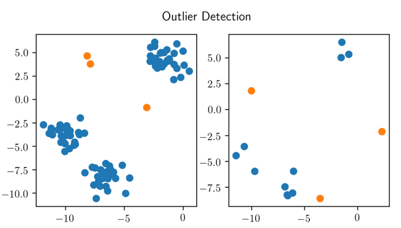
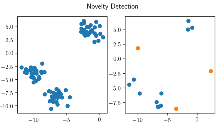
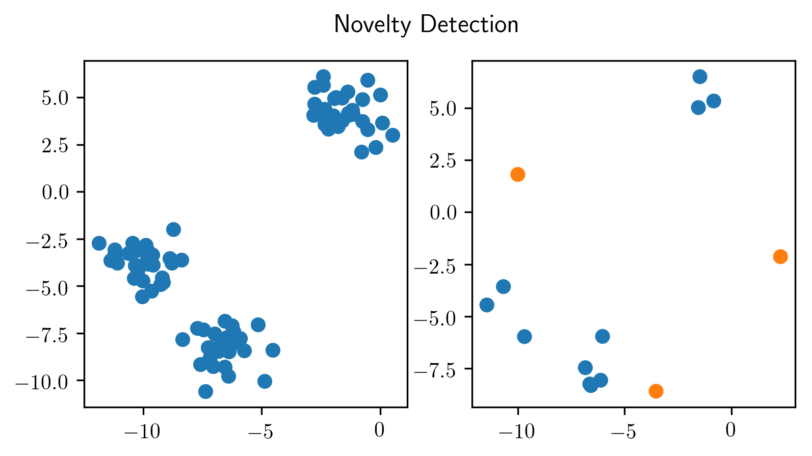
Both are unsupervised methods. The idea is to find things that are different. In outlier detection, usually, your training dataset also contains outliers which makes it a bit dirty, while in novelty detection, you get a dataset and then, later on, someone gives you new data and asks you what is new here. So in novelty detection, your dataset would be clean.
But in both, you want to identify something that’s sort of different from the standard distribution. Only, in the outlier detection case, there are already different samples in your training dataset.
This is one of the rigidly few unsupervised problems that are pretty heavily used in practice.
Find points that are “different” within the training set (and in the future).
“Novelty detection” - no outliers in the training set.
Outliers are not labeled! (otherwise it’s just imbalanced classification)
Often outlier detection and novelty detection used interchangeably in practice.
Applications
Fraud detection (credit cards, click fraud, …)
Network failure detection
Intrusion detection in networks
Defect detection (engineering etc…)
News? Intelligence?
usual assumption: all outliers are different in a different way.
Often people use classification datasets for outlier detection: that’s a bit strange. See homework results.
Basic idea
Model data distribution \(p(X)\)
–
Outlier: \(p(X) < \varepsilon\)
–
For outlier detection: be robust in modelling \(p(X)\)
The main idea is, you model your data distribution, p(X). And then you look at the data points that are unlikely under the model. So if it’s unlikely under the model, then it’s probably an outlier.
If you’re doing outlier detection that means your sample is going to be contaminated. So they’re outliers in the dataset X already if that is the case, you want to be robust in modeling p(X), so you want to model p(X) in a way that is robust to outliers.
Both of these tasks are generally ill-defined. So unless you actually know the real data distribution, how good something does is hard to measure. Usually, you don’t have ground truth of what the outliers are if you have the ground truth what the outliers are, you could just do an imbalance classification task.
So similar to clustering, what we’re doing here is building a model, trying to find some outliers, and then check if they’re actually outliers. If we are satisfied with the things that our model finds, then we can put into production. But there’s no guarantee that it’s going to find like x fraction of the outliers and since we don’t have labeled data, usually, we can’t really measure our recall. We won’t ever know about the samples that we didn’t find.
So maybe with respect to the homework and in the homework actually have ground truth data. And it’s similar to the clustering setting, where researchers are basically cheating and evaluating methods that are unsupervised in a supervised manner. So once you have ground truth label, you can evaluate your outlier detection, using, for example, AUC, which is what you’re going to do your homework.
But in a real-world setting, if you had the labels, you would never use outlier detection.
Again, similar to clustering, what makes an outlier in a particular dataset is ill-defined. So depends on the application, what do you want to consider an outlier or not. So in the homework, it’s ill and healthy, and the ill people are the outliers. But it could also be that the people that are much older and everybody else are the outliers.
If there’s sort of a very clear density model, and so you don’t know what the density of the data is supposed to look like and then, you know, things that don’t share this density, then you can sort of define this. But usually you don’t know what the density supposed to look like and so there’s no clearly defined notion of what is an outlier. Similarly only, there’s no clearly defined solution of what should be a cluster.
So we’re going to talk through a couple of different algorithms that make different assumptions about what makes a data point an outlier. So here, I said, we start usually with a data distribution p(X).
Task is generally ill-defined (unless you know the real data distribution).
Task is generally ill-defined (unless you know the real data distribution).
#Elliptic Envelope
.center[
 ]
]
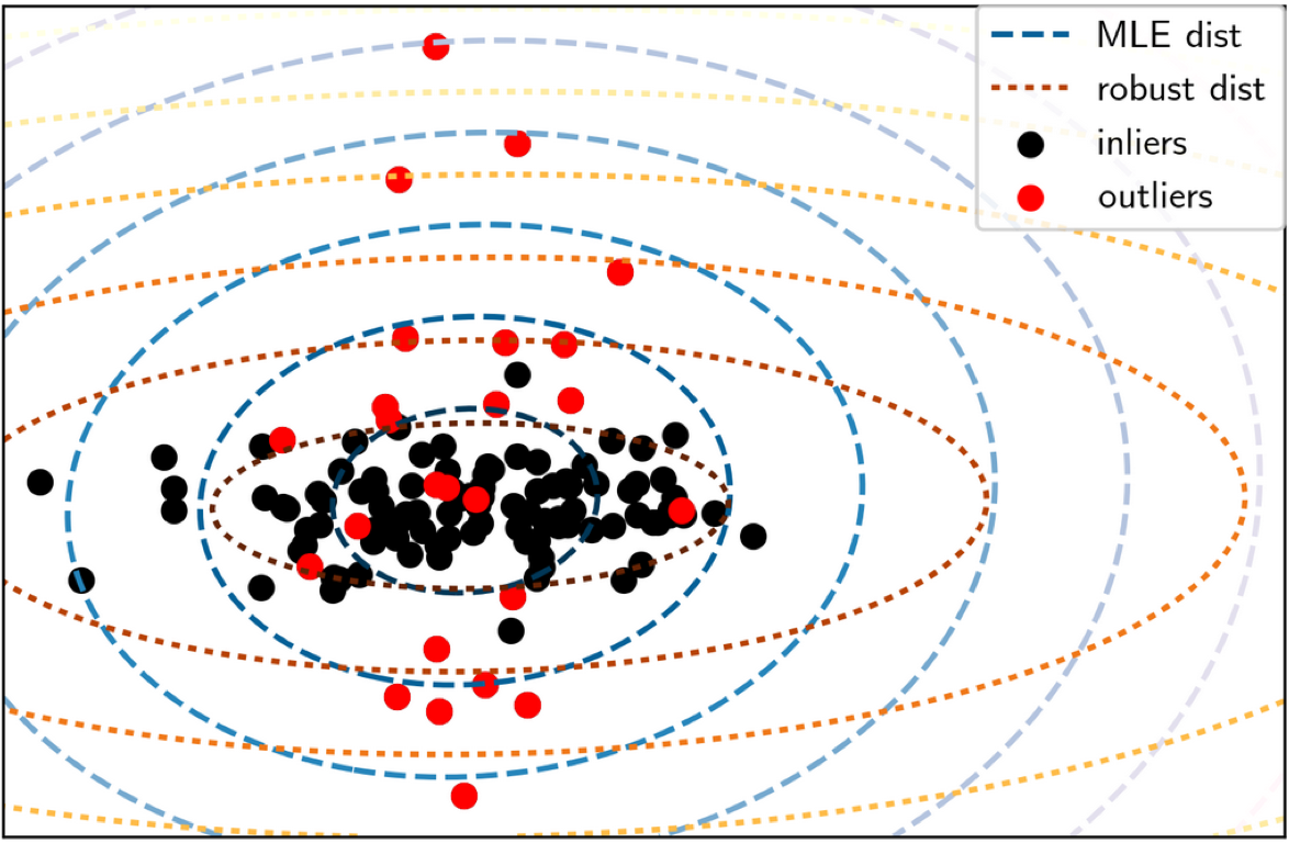
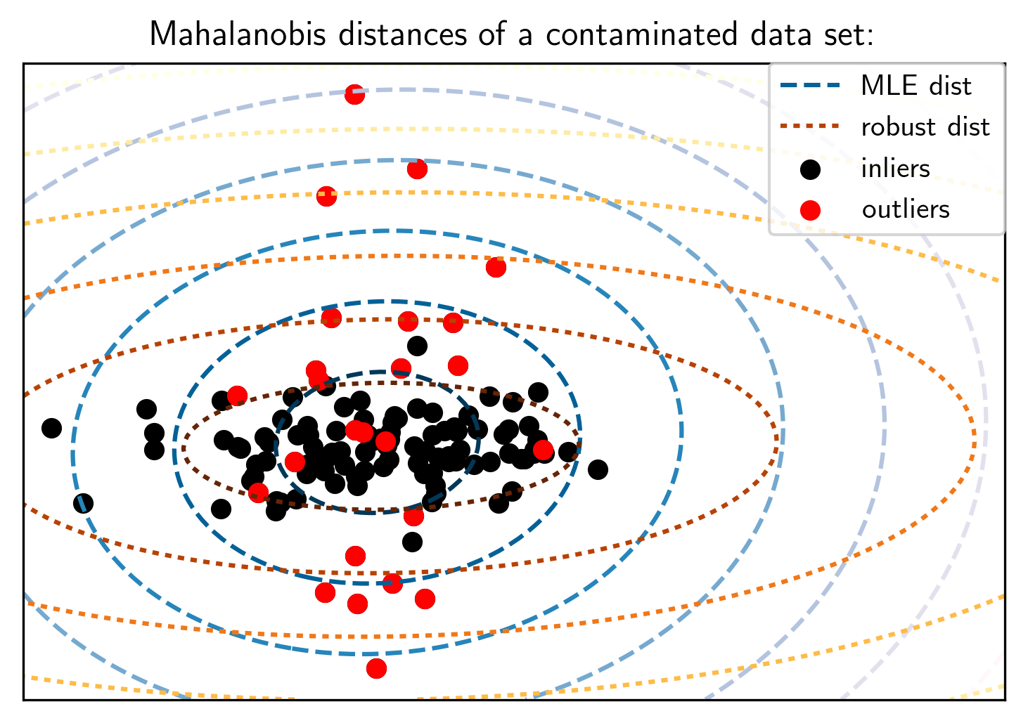
This leads to the elliptic envelope outlier detection. Basically, it fits a Gaussian into the data, and then it looks at the points that are not fit well by the Gaussians and those points are the outliers. Since this is meant for the outlier detection task, what we’re trying to do is actually trying to find a robust estimate of the mean and covariance matrix so that we can tolerate some outliers in the training dataset, and still sort of recover the real covariance matrix.
In this illustration, the black points, inliers, are what you expect the data to look like and the outlier distribution is plotted in red.
They overlap, so usually in unsupervised methods, you will never label any of these red points as outliers but we could try to figure out that these points here are outliers.
The way that elliptic envelope works are that it finds a robust version of the variance matrix. Basically, it finds the covariance matrix with the smallest determinant that still covers a large portion of the data.
In most outlier detection methods, you have to specify how many outliers you expect. So here, let’s say we specify 10% of the data to be outliers, then it will try to construct the covariance matrix that covers 90% of the data, but holds the lowest possible determinant.
If you do this, you get the red dotted circles, which are the contours covariance fitted with the robust estimate and the blue circles are the covariance fitted with the maximum likelihood estimates, using all the data.
Obviously, these outliers can disturb the covariance matrix and so the blue is sort of too thick in one direction whereas the red is not. So now, if you have this red model, you can basically say, all the data lies within these two standard deviations and so everything outside here is an outlier.
Fit robust covariance matrix and mean FIXME add slide on Covariance: Minimum Covariance Determination (MinCovDet)
Elliptic Envelope
Preprocessing with PCA might help sometimes.
.smaller[
from sklearn.covariance import EllipticEnvelope
ee = EllipticEnvelope(contamination=.1).fit(X)
pred = ee.predict(X)
print(pred)
print(np.mean(pred == -1))
```]

.smaller[
```python
[ 1  1  1  1  1  1  1  1  1  1  1  1  1  1  1  1  1  1  1  1  1  1  1  1  1
  1  1  1  1  1  1  1  1  1  1  1  1  1  1  1  1  1  1  1  1  1  1  1  1  1
  1  1  1  1  1  1  1  1  1  1  1  1  1  1  1  1  1  1  1  1  1  1  1  1  1
  1  1  1  1  1  1  1  1  1  1  1  1  1  1  1  1  1  1  1  1  1  1  1  1  1
 -1  1  1  1 -1 -1  1 -1  1  1 -1  1 -1 -1 -1  1  1 -1 -1 -1 -1  1 -1  1  1]
0.104

```]


The way we do this in scikit-learn. The covariance module
has all the robust covariance methods. As I said, you have
to specify the contamination, which is how many outliers do
you expect. Here, I set it to 10%.

If I predict I get 1s and -1s. All the outlier models in
scikit-learn use 1 for inliers and -1 to outliers.

The mean of the prediction tells me that about 10% of the
training data was labeled as an outlier, which is what we
would expect, given that we set it as 10%.  You could also
get a continuous score saying how much of an outlier is each
point with the score samples methods.

Here, in the elliptic envelope, contamination parameter
changes how the model is fit, for some other models, this
will actually only change the threshold. It’s important here
to have the right contamination parameters for the right
covariance fit.

For real-world model, set it based on what your expectations
are.
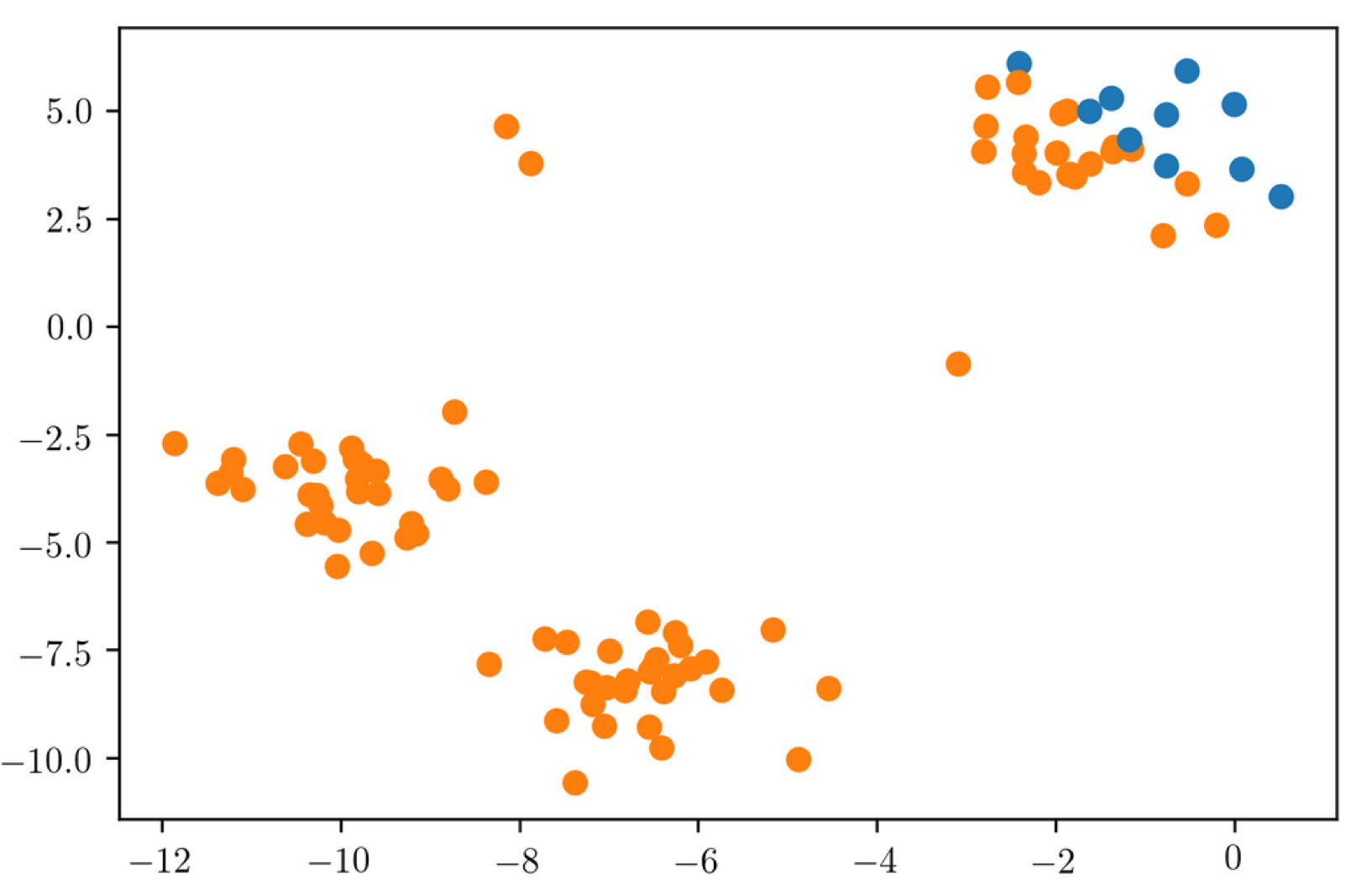
Failure-case: Non-Gaussian Data
.center[
 ]
]
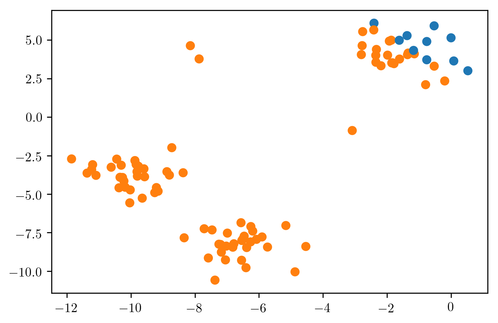
If the data is not Gaussian, we get this.
In this dataset, my intuition was that the isolated three points are the outliers and the rest are the normal data. Since the data is non-Gaussian, it gives you 10% as outliers that are furthest away from the mean. And this is not what I wanted at all.
So if your data is very non-Gaussian, then the method will not clearly work well.
Now, we could obviously use a more complicated density model. So we talked about Gaussian mixture models, we could use a Gaussian mixture model. Instead of fitting a single Gaussian, we could try to fit multiple Gaussian. If you just use the Gaussian mixture models in scikit-learn, they will not do a robust fit, so that might make more sense in the novelty detection than in the outlier detection sense because it will try to fit all of the data. You can still try to do it on the outlier detection task and just fit, so if I fit three Gaussians here, it’ll probably give me the right outliers. But then again, I need to know what the number of components is for my GMM, for this to work well.
So I still to make the assumptions about what the density is.
Another approach is instead of having a parametric density model like this, we can do a non-parametric density model like a kernel density estimate.
Could do mixtures of gaussians obviously!
Kernel Density
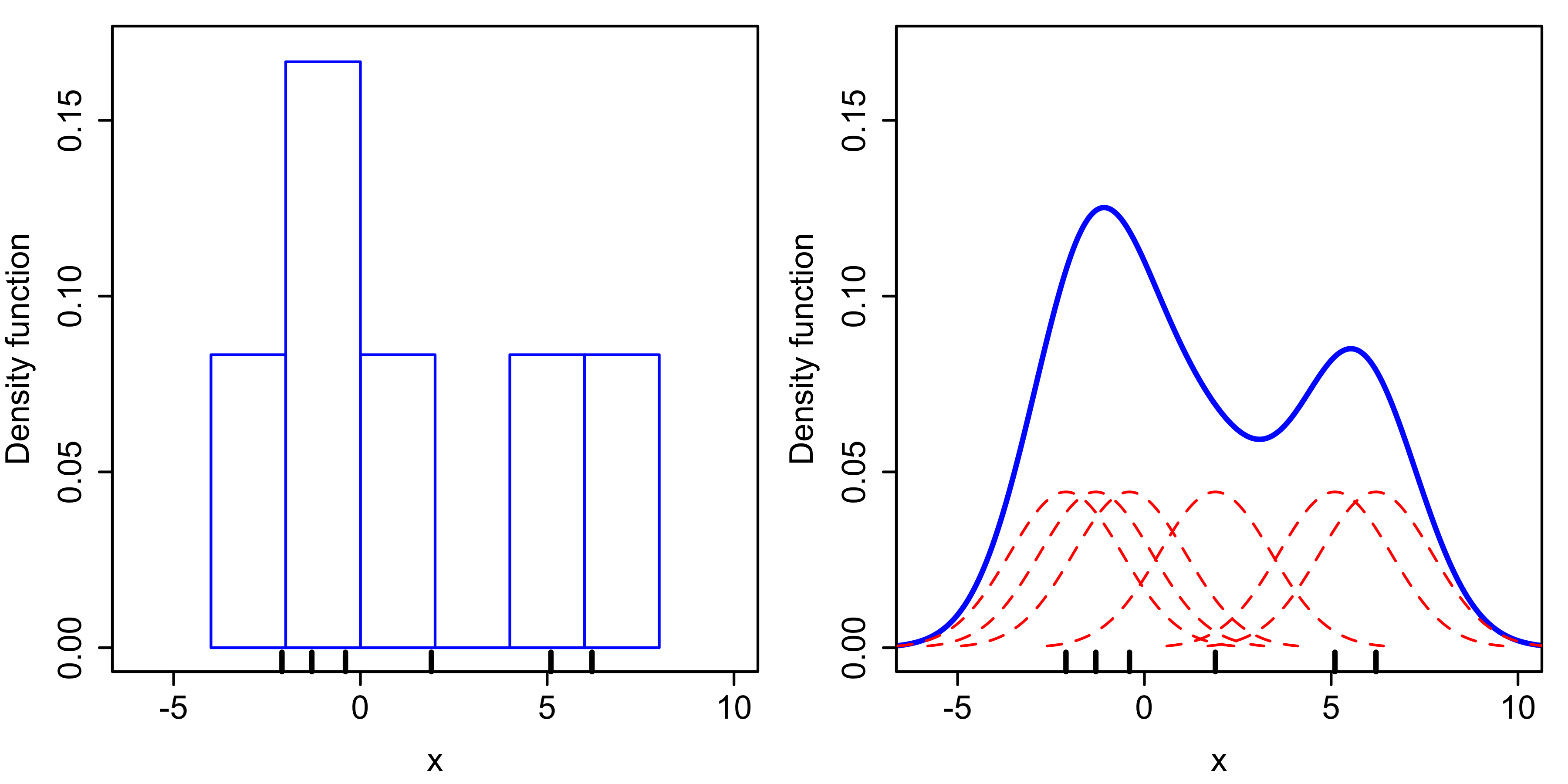
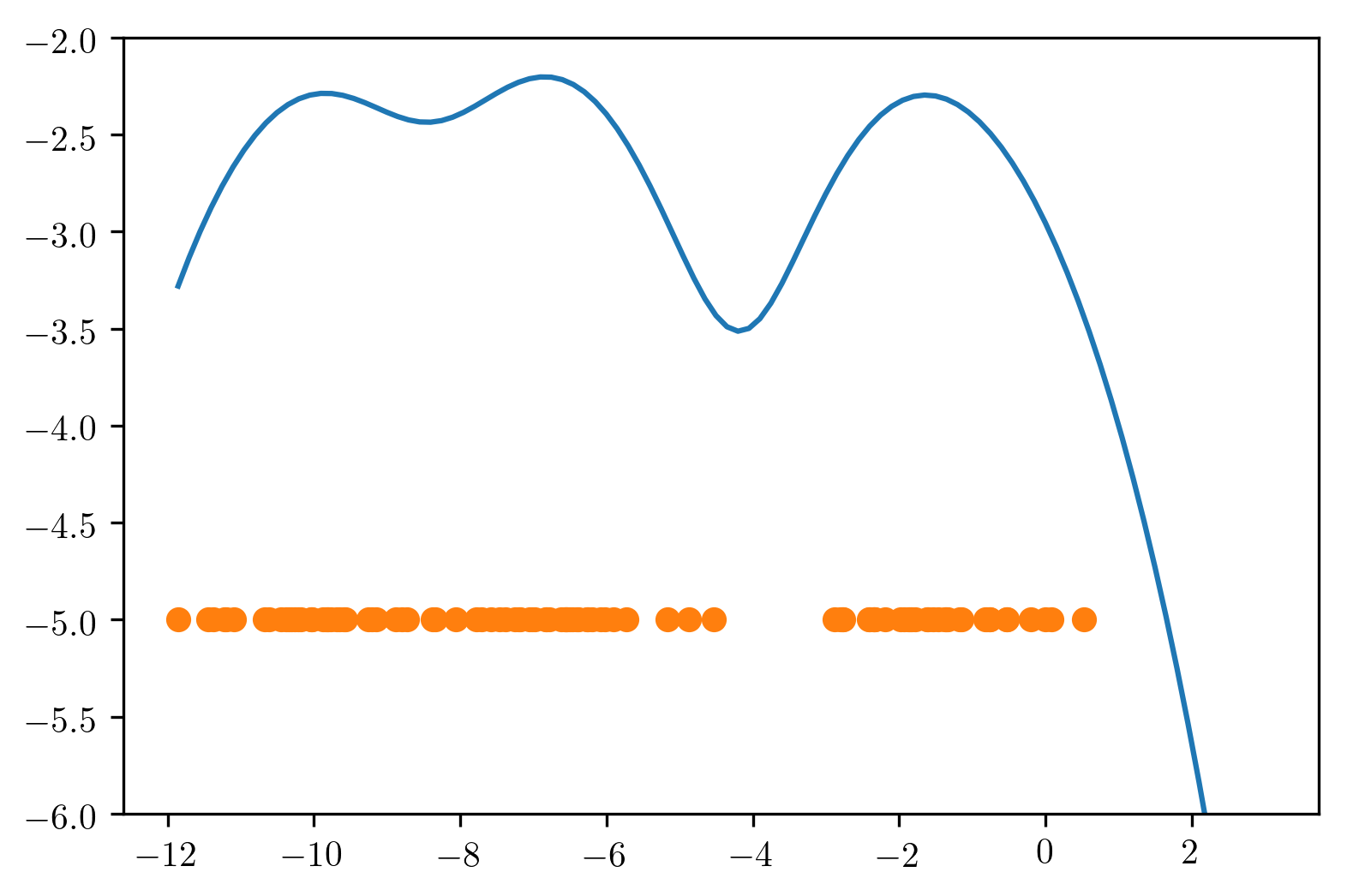
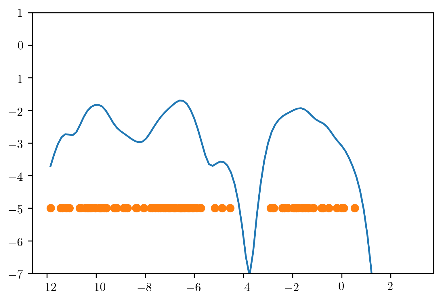
KDE is a most simple non-parametric estimate for probability distributions. The ticks at the bottom in the left plot are data points. One way to visualize the distribution is to do a histogram.
For the KDE estimate in the right, we put a small Gaussian blob around each data point. So here, each data point here at the bottom corresponds to one of these Gaussians and then we just sum them all up and this gives you sort of this smooth density here.
So this a little bit like a GMM where we have as many components as data points. You could also use other kernels.
The word kernel here means slightly different than in SVMs. Kernel here means kernel in the sense of signal processing. So another commonly used kernel here is the top hat kernel, which is a kernel in the signal processing sense but it’s not a kernel in the support vector machine sense, the Gaussian kernel was the kernel in both senses.
A kernel can mean a lot of different things. And here, it means basically windowing function. And so any windowing function would work for this, you kind of put a little bit of probability math around each data point.
An obvious problem with this is that you need to pick the bandwidth.
Non-parametric density model
Gaussian blob on each data point
Doesn’t work well in high dimensions
Kernel Bandwidth
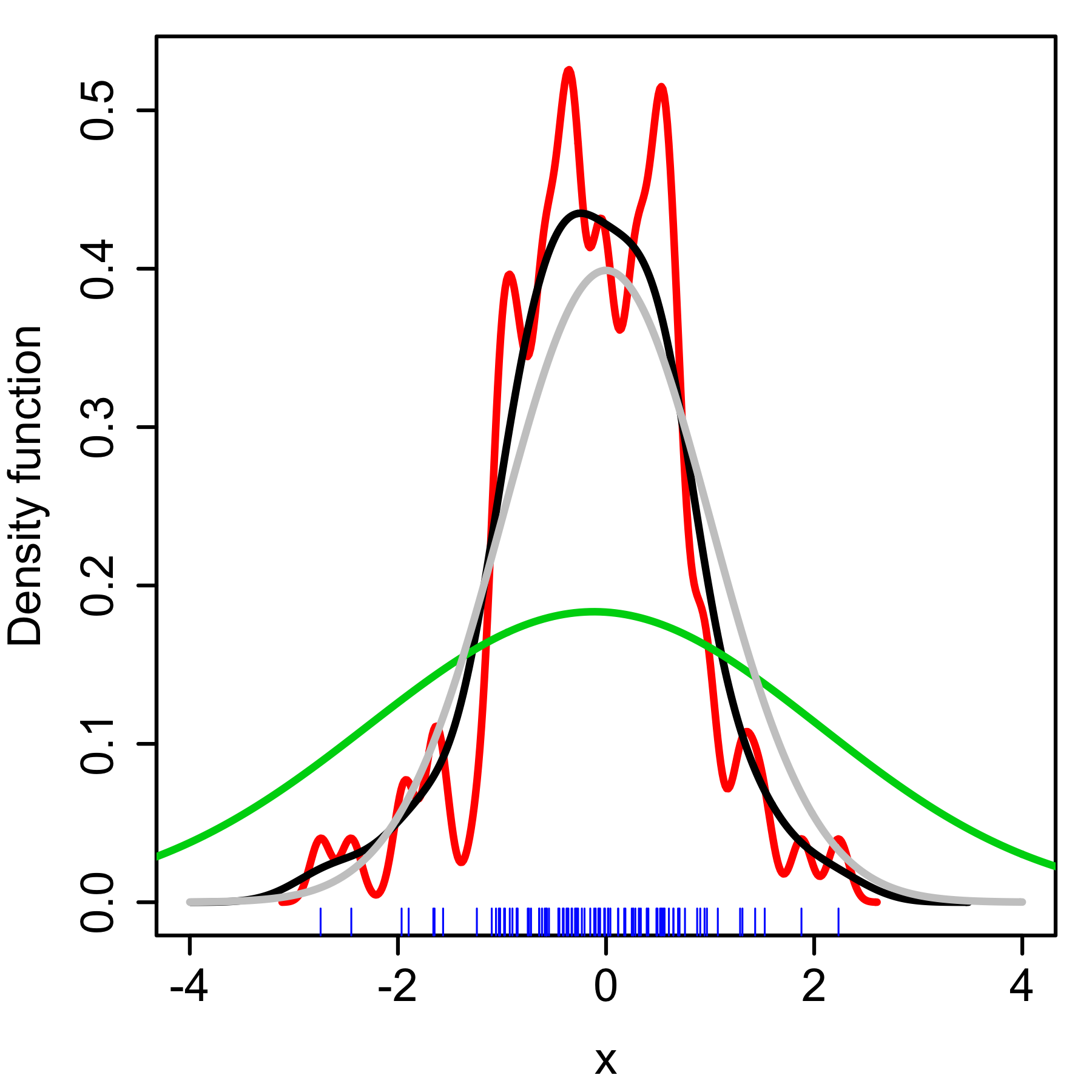
So depending on what bandwidth you pick, you can either over smooth or under smooth the data. Here, in red, you’ve picked too small of bandwidth while in green, you’ve picked two large of bandwidth and black is probably a decent bandwidth.
Again, this is an unsupervised problem. So it’s very hard to do this. You can actually use cross validation to adjust the bandwidth. So you can look at what’s the score of the held out data.
This is also not a robust estimate. So if you have outliers in your data, the outliers in your data might influence your estimate.
The other problem with this is that KDDs don’t work in higher dimensions. You can obviously not only do this 1-dimension, but you can also do this in any number of dimensions. But here, you get the curse of dimensionality. Basically, if you have higher dimensional space, you need more and more data points to actually fill the space with these small Gaussian blobs. If you would want to do a histogram, in like 10 dimensions, and you don’t have enough data, then most of the histogram cells will be empty. And here, this is only like a smooth version of the histogram so it has the same problem.
So if your space is in high dimensional, most of the space will be empty and this is not going to work very well.
Need to adjust kernel bandwidth
Unsupervised model, so how to pick kernel bandwidth?
cross-validation can be used to pick the bandwidth, but if there’s outliers in the training data, could go wrong?
.smaller[
kde = KernelDensity(bandwidth=3)
kde.fit(X_train_noise)
pred = kde.score_samples(X_train_noise)
pred = (pred > np.percentile(pred, 10)).astype(int)
```]
.center[

]
If your space is low dimensional, and you can plot it, it
might work nicely. So here, I might have used the
cross-validation to find out the bandwidth of 3 is good. And
then I can look at the scores. So here, KDE is not an
outlier detection method in scikit-learn, but I can use it
as an outlier detection method by just looking at score
samples, which are the log probabilities of all the data
points under this probability model. And I say that
everything that's higher than the 10th percentile is an
inlier.
So basically, now I label 10% of the data as outliers and I
actually get the right three points that I wanted and a
couple more points. Obviously, I get more points, because I
told them I want 10% of my data to be outliers.
So this is a really is a very simple method. But it doesn’t
work well in higher dimensions and it gets very slow since
you have a lot of these kernels that you need to evaluate.
So you need to compute the distance between all pairs of
points mostly.
One Class SVM
Also uses Gaussian kernel to cover data
Only select support vectors (not all points)
Specify outlier ratio (contamination) via nu
.smaller[
from sklearn.svm import OneClassSVM
scaler = StandardScaler()
X_train_noise_scaled = scaler.fit_transform(X_train_noise)
oneclass = OneClassSVM(nu=.1).fit(X_train_noise_scaled)
pred = oneclass.predict(X_train_noise_scaled)
```]
A more sophisticated variant of this is the one class SVM.
This also uses Gaussian kernels to basically cover the data.
But it selects only support vectors, not all points as basis
points. You get a similar function, in KDE.
But the density function is supported only by some support
vectors. Again, you need to specify the bandwidth parameter
gamma. So this only makes sense with an RVF kernel. It’s
quite similar to what KDE does, but only, it selects support
vectors and does it in a more robust way.
You also have to set the number of outliers you expect as
nu. Again, nu is part of the optimization process. So
setting the outlier fraction differently will change how the
models fit.
- Need to adjust kernel bandwidth
- nu is "training mistakes"
+++
.center[

]
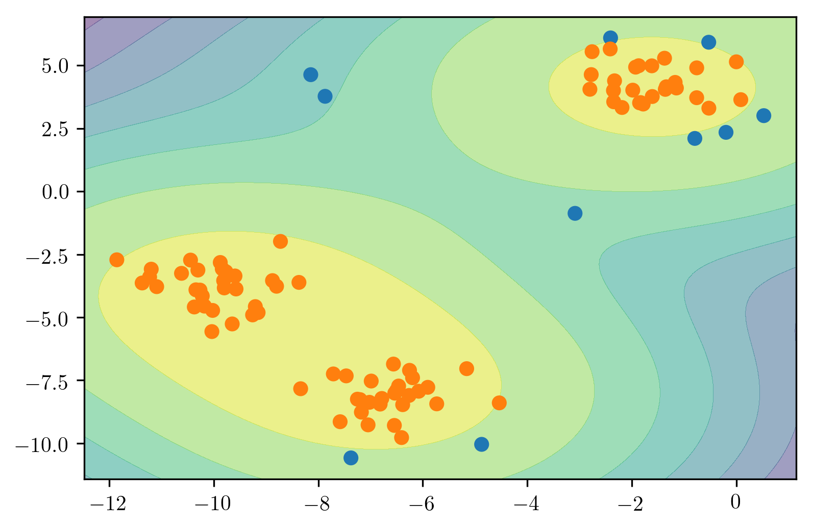
So here, this was with a particular setting of gamma, and
you can see that it seems like a somewhat reasonable model.
If I made gamma a little bit smaller, it would probably have
found the right points. But here, it's even harder to adjust
the gamma parameter because there's no way to really do it.
So for KDE, I can do cross-validation to see how good of a
probability model this is, while the SVM doesn't have a
probability model. So I can't do cross-validation or
anything. So I just need to pick gamma in some way that
makes sense to me, which is not great.
If you can visualize data, obviously, that helps. But in
higher dimensions, you need to look at projections or other
things to see how to set gamma. So in a sense, is also sort
of a non-parametric density estimate. But it doesn't really
have a probabilistic model.
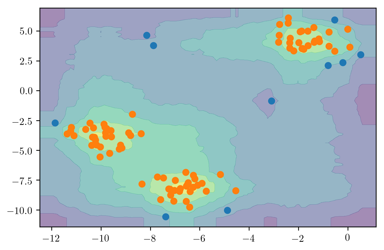
Isolation Forests
The final model I want to talk about is also a non-parametric estimate that also doesn’t have a probability model and it’s called isolation forest
By far, it’s my favorite since it has no parameters to tune.
#Idea
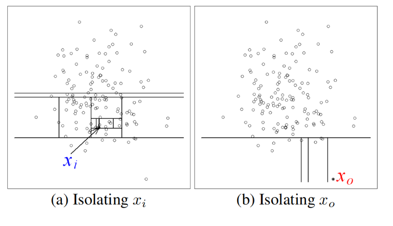
Outliers are easy to isolate from the rest
.center[
 ]
]
So the idea of isolation forest is that if you build a random tree over a dataset, then if you want to figure out how easy is it to split up a particular point, it’s much easier to split up a point that’s an outlier, that’s on the outside of the data than a point that’s like somewhere where the data is very dense.
The idea is that you build many completely random trees, it’s complete unsupervised, so it just keeps splitting the data in some way and we look at how deep do we need to go to isolate a data point from the other data points.
If on average, we have to go very deep into the tree, it’s probably if some of our data is dense, it’s not an outlier. So on average, if we split off the point very early, it’s probably an outlier.
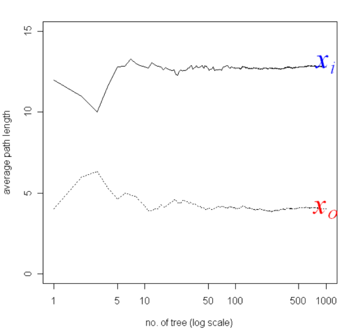
Measure as Path length!
.left-column[
]
.right-column[
 ]
]
If you add more and more completely random trees, you get a relatively stable score that tells you is it an outlier or is it an outlier. You can think of this as sort of trying to model the density of the data. But there’s no probabilistic model here.
X1 has over 1000 trees, you need a very long path line so you go very deep into a tree before it’s isolated from the other point. That means it’s in a very dense region. Whereas, X0, on average is split up quite early from the rest of data points so it’s probably an outlier. So basically, if you’re on the outside of the data, no matter what feature is picked, you’re likely to be split off, given that you’re an outlier with respect to any of these features.
#Normalizing the Path Length
Average path length of unsuccessful search in Binary Search Tree:
s < 0.5 : definite inlier
s close to 1: outlier
So to make this more coherent, we need to normalize the path lines. And so depending on how many data points there are, you expect to go deeper to the tree to separate something. And so you can calculate what the average path length of an unsuccessful search is in the binary tree, which is similar to trying to isolate a point, and you can compute this number.
And the score that we actually compute, the outlier score is 2 to the minus average path length over all the trees divided by the average path lengths for an unsuccessful search in binary trees. So this only depends on n which is the number of data points. So basically, we are only normalizing the score to make sense independent of the dataset size.
If this score is smaller than 0.5 then definitely you’re an inlier. If it’s closer to 1, it’s an outlier.
Basically, the way you determine outliers is by threshold the score. So here, setting the number of expected outliers doesn’t change the algorithm at all, it only changes the threshold for this core function. So here, picking the number of outliers in advance is not as important.
Building the forest
Subsample dataset for each tree
Default sample size of 256 works surprisingly well
Stop growing tree at depth log_2(sample size) – so 8
No bootstrapping
More trees are better – default 100
Need to specify contamination rate
It has no parameters, it’s quite simple to do this. So what we’re doing is actually we subsample the dataset for each tree and we picked 256 samples. The default value of 256 samples always works, no matter what the dataset size is. And we stopped growing the tree at depth log_2 (sample size), which is 8.
So you repeatedly draw, without replacement, 256 samples from your data and grow trees of depth 8 and then you look at the average path length to isolate a point.
Obviously, as with all random forest, more trees are better but the default in scikit-learn is 100.
In principle, these are free parameters of the algorithm, like, how much to subsample for each tree, and how to prune each tree. But people don’t tune these parameters and it just works well.
The contamination rate only picks the threshold on this final score.
FIXME all the text
.center[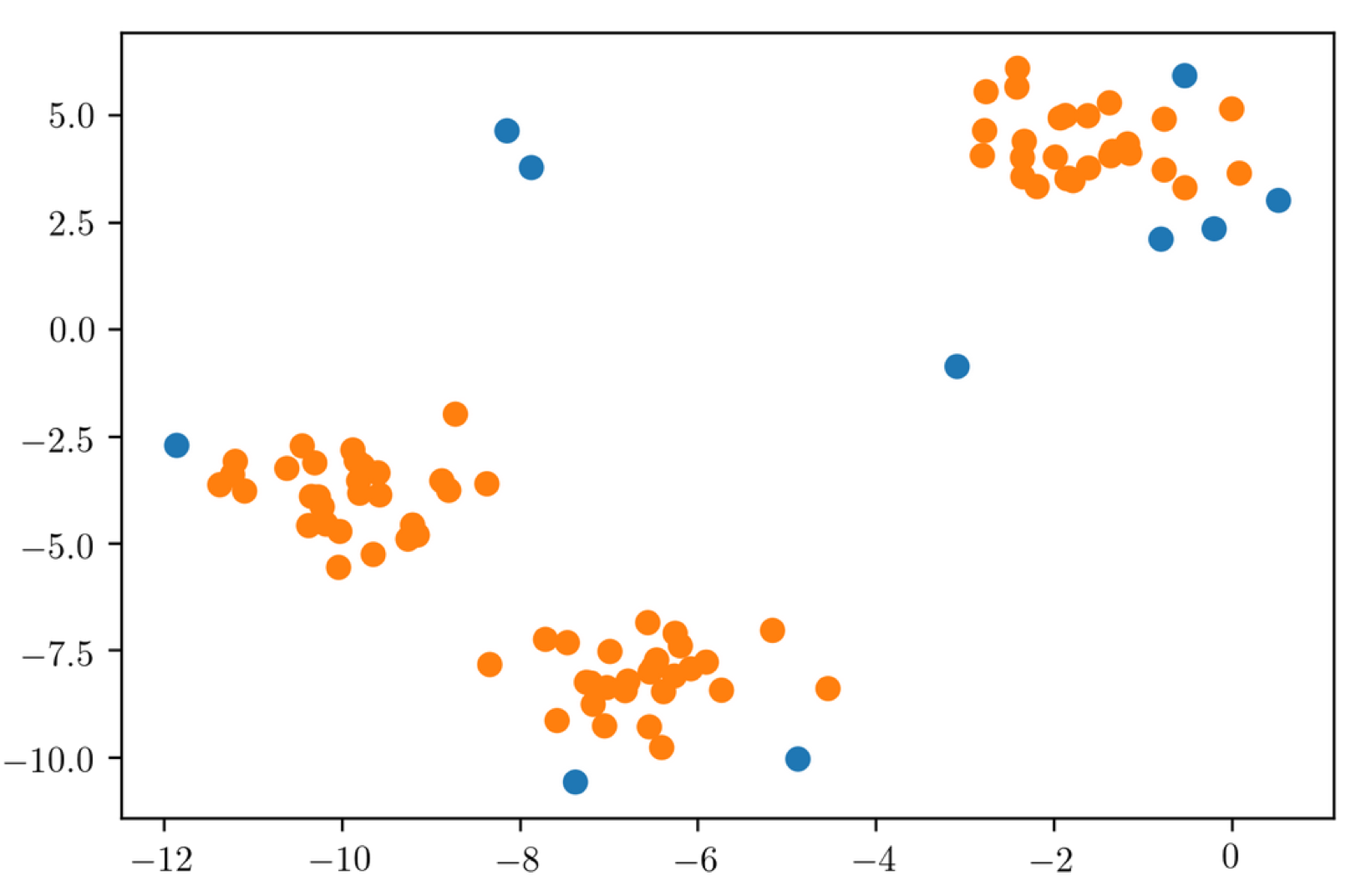 ]
]
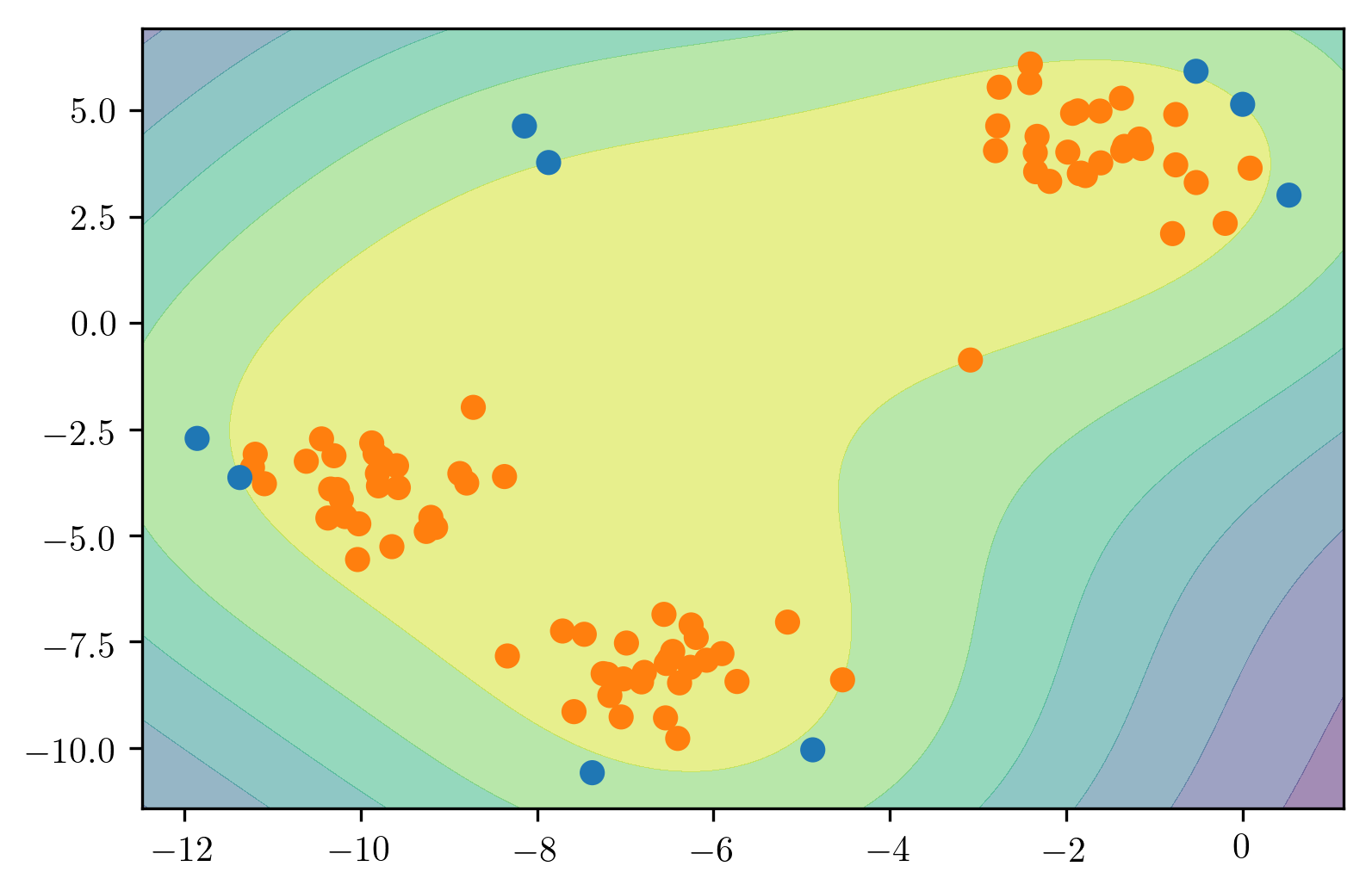
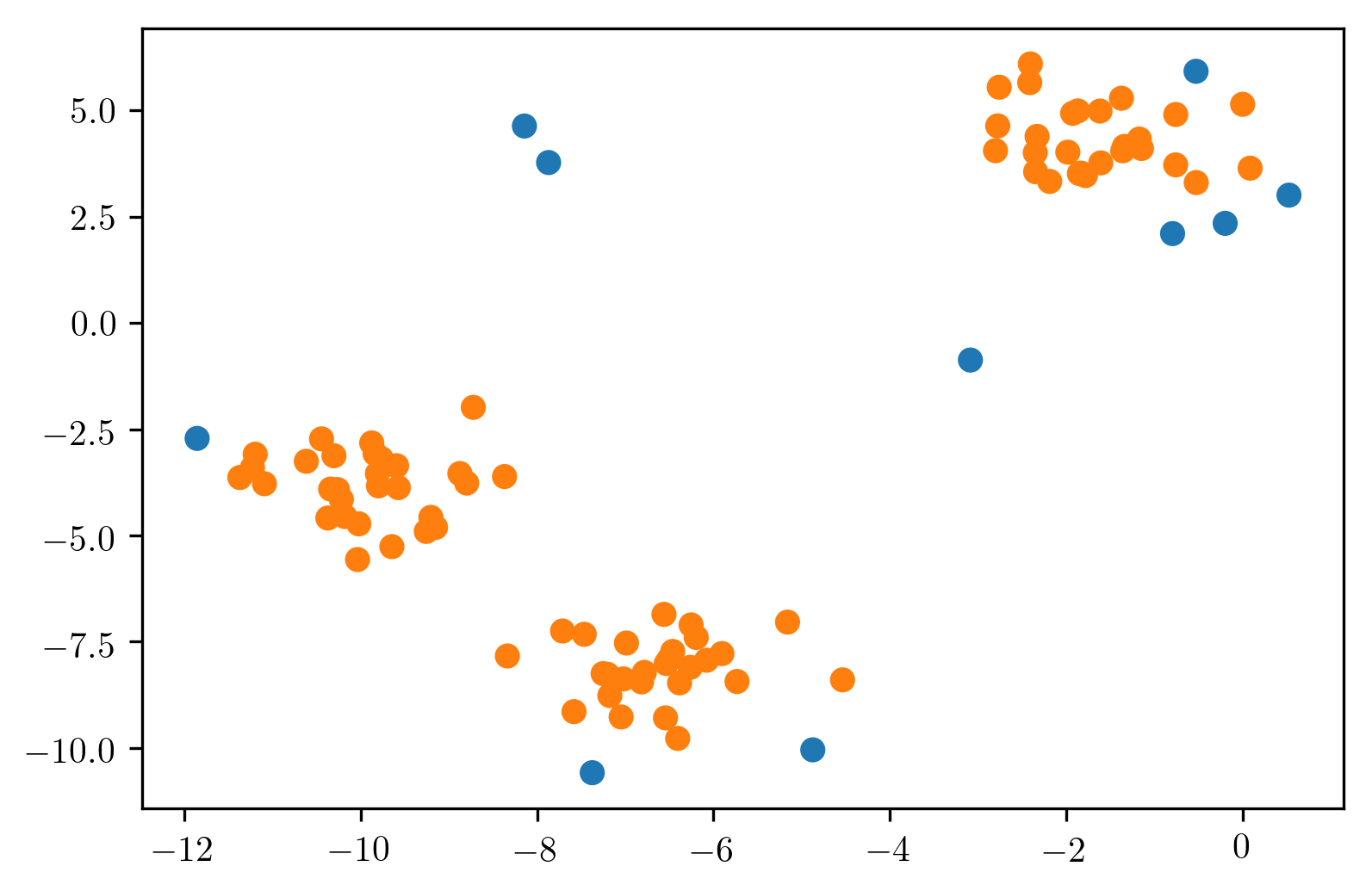
Here is what the algorithm produces and it worked as good as I thought.
Remember, this is a toy dataset. It doesn’t really tell you that much about how works in the real world.
.center[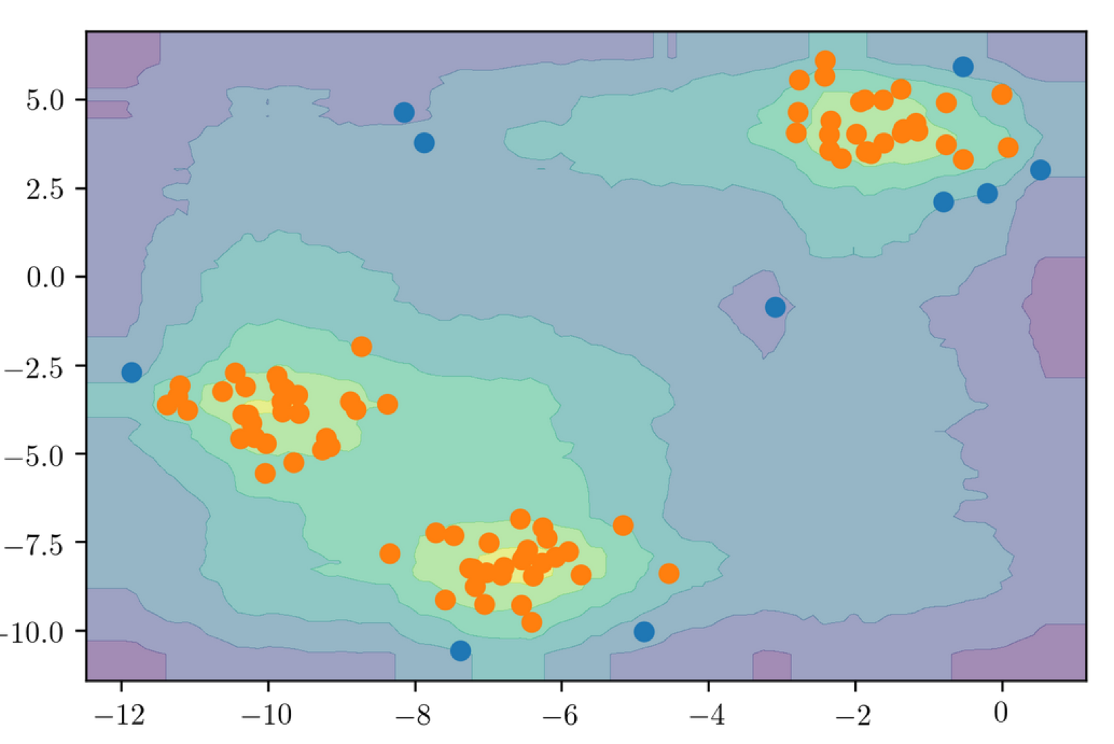 ]
]
Here, I plotted the score for each data point. You could do this for data models too. Here, since it’s tree-based, it’s not nice and smooth as it is for support vector machine or the KDE. I didn’t have to tune any kernel bandwidth or anything and so that’s kind of nice.
Again, it also depends on what your assumptions are about outliers. This will not work very well for the homework. And you can think about why this does not work very well from your homework.
Other density based-models
PCA
GMMs
Robust PCA (not in sklearn :-()
Any other probabilistic model - “robust” is better.
You can use other density based models. You can use just PCA which is also like a higher dimensional Gaussian model in some sense, where you drop some of the directions.
You can use GMMs.
There’s a robust variant of PCA that is, unfortunately, not on scikit-learn.
You can use any probabilistic model that you want. But you need to think about if the model is appropriate for the data that you’re trying to model. And if you expect there’s a lot of outliers in your training dataset already, then you might need to think about how to make the model robust.
So PCA is not robust, while robust PCA is robust. And so if you have very big outliers in your dataset, it will skew your PCA results and so that might not work as well.
robust only needed for outlier detection, not novelty detection.
.center[
 ]
]
.center[
 ]
]
.center[
 ]
]
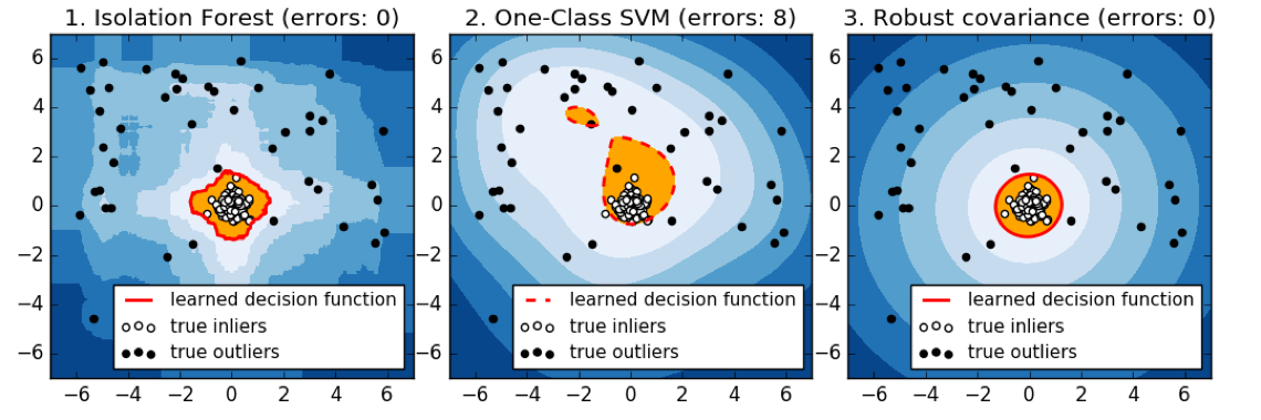
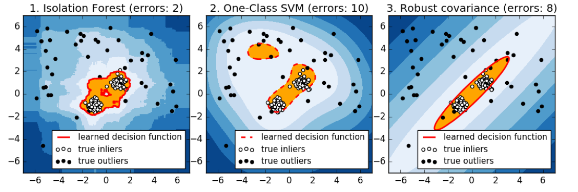
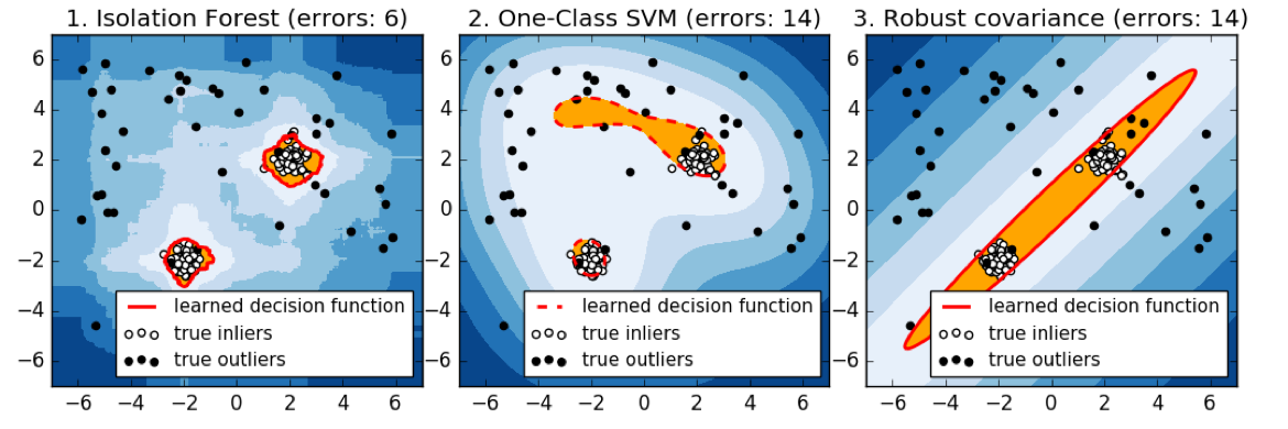
Here is a comparison of the three of the four models that we talked about. So here, we’re looking at isolation forest, one class SVM, and robust covariance.
Basically, the robots covariance works perfectly for isotropic Gaussian, because that’s what it fits. If you have multiple Gaussians it kind of breaks down. So if they’re close enough together, maybe it makes sense to model them as joint Gaussian. But if you put them further apart, basically, it will change the covariance shape and so it will have a bad model of your data.
So the isolation forest does kind of reasonably well in all cases. I mean, this is a 2D dataset and so it can just find dense regions without a problem. Whereas the one class SVM, gives slightly strange results, probably because it picked some support vectors to cover the data.
Ideally, the one class SVM is supposed to be robust to contamination in the training set, but as we can see, it’s not that robust to contamination. The one clause SVM might work better when you have a clean training dataset.
There’s no definition of true outliers, obviously. But here, we have drawn very densely from either one or two Gaussian models, the inliers are white and then we have random uniform over this whole square some outliers.
The idea is basically, there’s 3 different distribution that the data is drawn from. There’s like some Gaussian points and some points that are just uniform. And you want to isolate the very dense points from the uniform that not very dense points.
Summary
Isolation Forest works great!
Density models are great if they are correct.
Estimating bandwidth can be tricky in the unsupervised setting.
Validation of results often requires manual inspection.
As with all unsupervised methods, for outlier detection, validating the model and tuning the parameters are really hard. So the more your model depends on parameters, like the one class SVM depends a lot on parameters, it’s just very tricky to do that.
As with the clustering, validation often means looking into the data, looking at single data points, why are they outliers and trying to interpret the results. Because if you have two labels, why don’t you learn a classifier.
One possible approach that I didn’t talk about is if you have a big dataset that’s not labeled, you can run an outlier detection algorithm, you can find like 10% most outlier things according to your algorithm, you can confirm manually whether they are outliers or not and then you could run a classifier. It depends a little bit on whether the outliers are all outliers in a similar way or outliers in different ways. So if all your outliers are outliers in a different way, then running a classifier will actually not work. So in that setting, you might actually be better off with an outlier detection method.
Even if you have labels, if all of your outliers are outliers in a very different way, it might be better to just build the model off the non-outlier data and then call everything else that’s an outlier instead of trying to learn a classifier. If there’s no dense region of outliers, then you can’t learn a classifier for that.
import numpy as np
import matplotlib.pyplot as plt
% matplotlib inline
plt.rcParams["figure.dpi"] = 300
np.set_printoptions(precision=3, suppress=True)
import pandas as pd
from sklearn.model_selection import train_test_split, cross_val_score
from sklearn.pipeline import make_pipeline
from sklearn.preprocessing import scale, StandardScaler
from matplotlib.offsetbox import OffsetImage, AnnotationBbox
from sklearn.datasets import fetch_mldata
mnist = fetch_mldata("MNIST original")
/home/andy/checkout/scikit-learn/sklearn/utils/deprecation.py:76: DeprecationWarning: Function fetch_mldata is deprecated; fetch_mldata was deprecated in version 0.20 and will be removed in version 0.22. Please use fetch_openml.
  warnings.warn(msg, category=DeprecationWarning)
/home/andy/checkout/scikit-learn/sklearn/utils/deprecation.py:76: DeprecationWarning: Function mldata_filename is deprecated; mldata_filename was deprecated in version 0.20 and will be removed in version 0.22. Please use fetch_openml.
  warnings.warn(msg, category=DeprecationWarning)
---------------------------------------------------------------------------
ConnectionResetError                      Traceback (most recent call last)
<ipython-input-3-8a029c5f792a> in <module>()
      1 from sklearn.datasets import fetch_mldata
----> 2 mnist = fetch_mldata("MNIST original")

~/checkout/scikit-learn/sklearn/utils/deprecation.py in wrapped(*args, **kwargs)
     75         def wrapped(*args, **kwargs):
     76             warnings.warn(msg, category=DeprecationWarning)
---> 77             return fun(*args, **kwargs)
     78
     79         wrapped.__doc__ = self._update_doc(wrapped.__doc__)

~/checkout/scikit-learn/sklearn/datasets/mldata.py in fetch_mldata(dataname, target_name, data_name, transpose_data, data_home)
    124         urlname = MLDATA_BASE_URL % quote(dataname)
    125         try:
--> 126             mldata_url = urlopen(urlname)
    127         except HTTPError as e:
    128             if e.code == 404:

~/anaconda3/envs/py37/lib/python3.7/urllib/request.py in urlopen(url, data, timeout, cafile, capath, cadefault, context)
    220     else:
    221         opener = _opener
--> 222     return opener.open(url, data, timeout)
    223
    224 def install_opener(opener):

~/anaconda3/envs/py37/lib/python3.7/urllib/request.py in open(self, fullurl, data, timeout)
    523             req = meth(req)
    524
--> 525         response = self._open(req, data)
    526
    527         # post-process response

~/anaconda3/envs/py37/lib/python3.7/urllib/request.py in _open(self, req, data)
    541         protocol = req.type
    542         result = self._call_chain(self.handle_open, protocol, protocol +
--> 543                                   '_open', req)
    544         if result:
    545             return result

~/anaconda3/envs/py37/lib/python3.7/urllib/request.py in _call_chain(self, chain, kind, meth_name, *args)
    501         for handler in handlers:
    502             func = getattr(handler, meth_name)
--> 503             result = func(*args)
    504             if result is not None:
    505                 return result

~/anaconda3/envs/py37/lib/python3.7/urllib/request.py in http_open(self, req)
   1343
   1344     def http_open(self, req):
-> 1345         return self.do_open(http.client.HTTPConnection, req)
   1346
   1347     http_request = AbstractHTTPHandler.do_request_

~/anaconda3/envs/py37/lib/python3.7/urllib/request.py in do_open(self, http_class, req, **http_conn_args)
   1318             except OSError as err: # timeout error
   1319                 raise URLError(err)
-> 1320             r = h.getresponse()
   1321         except:
   1322             h.close()

~/anaconda3/envs/py37/lib/python3.7/http/client.py in getresponse(self)
   1319         try:
   1320             try:
-> 1321                 response.begin()
   1322             except ConnectionError:
   1323                 self.close()

~/anaconda3/envs/py37/lib/python3.7/http/client.py in begin(self)
    294         # read until we get a non-100 response
    295         while True:
--> 296             version, status, reason = self._read_status()
    297             if status != CONTINUE:
    298                 break

~/anaconda3/envs/py37/lib/python3.7/http/client.py in _read_status(self)
    255
    256     def _read_status(self):
--> 257         line = str(self.fp.readline(_MAXLINE + 1), "iso-8859-1")
    258         if len(line) > _MAXLINE:
    259             raise LineTooLong("status line")

~/anaconda3/envs/py37/lib/python3.7/socket.py in readinto(self, b)
    587         while True:
    588             try:
--> 589                 return self._sock.recv_into(b)
    590             except timeout:
    591                 self._timeout_occurred = True

ConnectionResetError: [Errno 104] Connection reset by peer
X = mnist.data / 255.

from sklearn.decomposition import NMF, PCA
pca = PCA(n_components=4)
pca.fit(X)
PCA(copy=True, iterated_power='auto', n_components=4, random_state=None,
  svd_solver='auto', tol=0.0, whiten=False)
def plot_decomposition(image, components, coef, cmap='viridis'):
    image_shape = image.shape
    plt.figure(figsize=(20, 3))
    ax = plt.gca()


    imagebox = OffsetImage(image, zoom=5, cmap="gray")
    ab = AnnotationBbox(imagebox, (.05, 0.4), pad=0.0, xycoords='data')
    ax.add_artist(ab)
    sorting = np.argsort(np.abs(coef))[::-1]

    for i in range(4):
        imagebox = OffsetImage(components[sorting[i]].reshape(image_shape), zoom=5., cmap=cmap)


        ab = AnnotationBbox(imagebox, (.3 + .2 * i, 0.4),
                          pad=0.0,
                          xycoords='data'
                          )
        ax.add_artist(ab)
        if i == 0:
            plt.text(.18, .3, r'{:.2f}'.format(coef[sorting[i]]), fontdict={'fontsize': 30})
        else:
            plt.text(.165 + .202 * i, .3, r'+ {:.2f}'.format(coef[sorting[i]]), fontdict={'fontsize': 30})

    plt.text(.96, .25, '+ ...', fontdict={'fontsize': 30})

    plt.rc('text', usetex=True)
    plt.text(.13, .3, r'\approx', fontdict={'fontsize': 30})
    plt.axis("off")
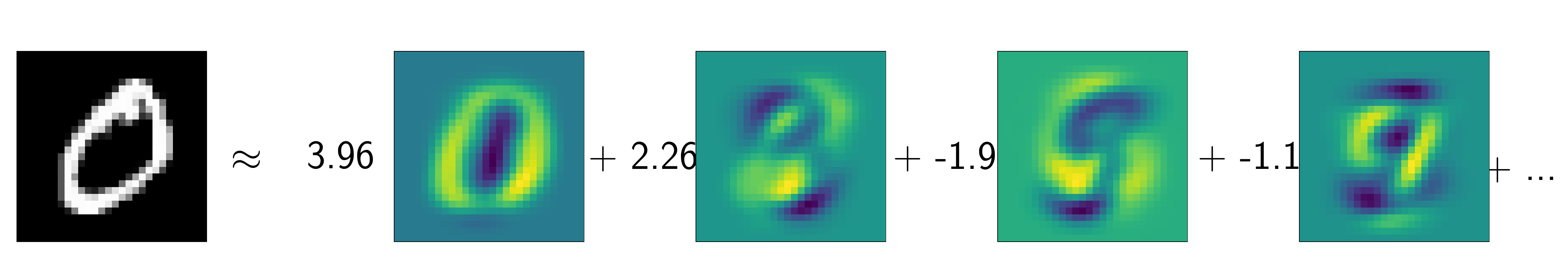
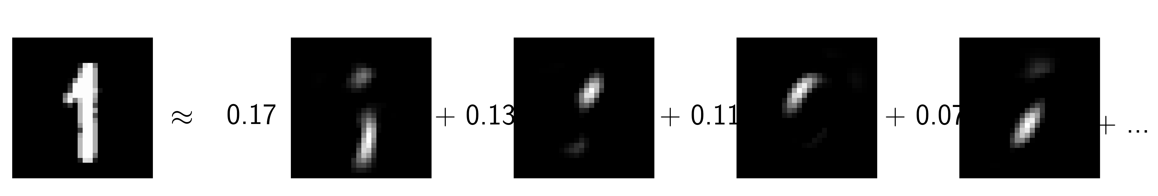
plot_decomposition(mnist.data[0].reshape(28, 28), pca.components_, pca.transform(mnist.data[:1] / 255.)[0])
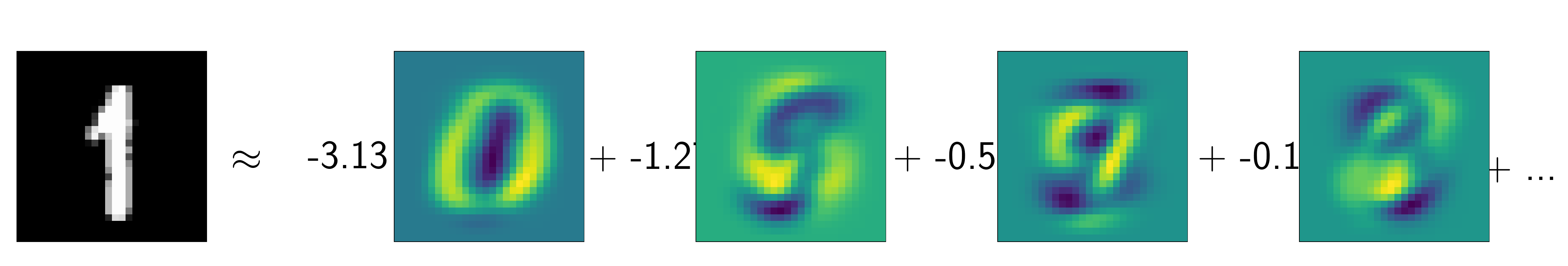
plot_decomposition(mnist.data[11000].reshape(28, 28), pca.components_, pca.transform(mnist.data[11000:11001] / 255.)[0])
nmf = NMF(n_components=20)
nmf.fit(X)
NMF(alpha=0.0, beta_loss='frobenius', init=None, l1_ratio=0.0, max_iter=200,
  n_components=20, random_state=None, shuffle=False, solver='cd',
  tol=0.0001, verbose=0)
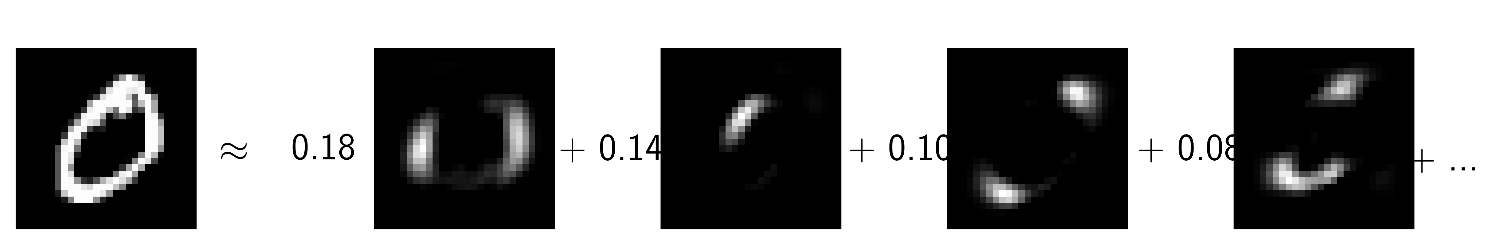
plot_decomposition(mnist.data[0].reshape(28, 28), nmf.components_, nmf.transform(mnist.data[:1] / 255.)[0], cmap="gray")
plot_decomposition(mnist.data[11000].reshape(28, 28), nmf.components_, nmf.transform(mnist.data[11000:11001] / 255.)[0], cmap="gray")
nmf20 = NMF(n_components=20)
nmf20.fit(X)
NMF(alpha=0.0, beta_loss='frobenius', init=None, l1_ratio=0.0, max_iter=200,
  n_components=20, random_state=None, shuffle=False, solver='cd',
  tol=0.0001, verbose=0)
nmf5 = NMF(n_components=5)
nmf5.fit(X)
NMF(alpha=0.0, beta_loss='frobenius', init=None, l1_ratio=0.0, max_iter=200,
  n_components=5, random_state=None, shuffle=False, solver='cd',
  tol=0.0001, verbose=0)
fig, axes = plt.subplots(4, 5, figsize=(10, 5))
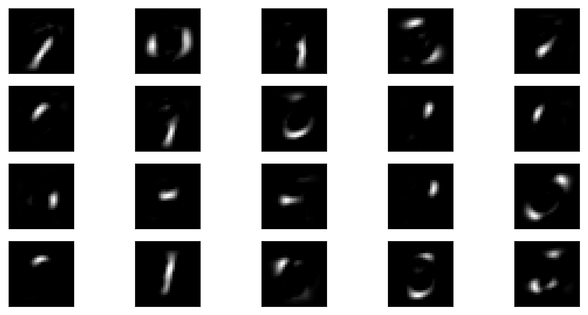
for ax, comp in zip(axes.ravel(), nmf20.components_):
ax.imshow(comp.reshape(28, 28), cmap="gray")
ax.set_xticks(())
ax.set_yticks(())
fig, axes = plt.subplots(1, 5, figsize=(10, 5))
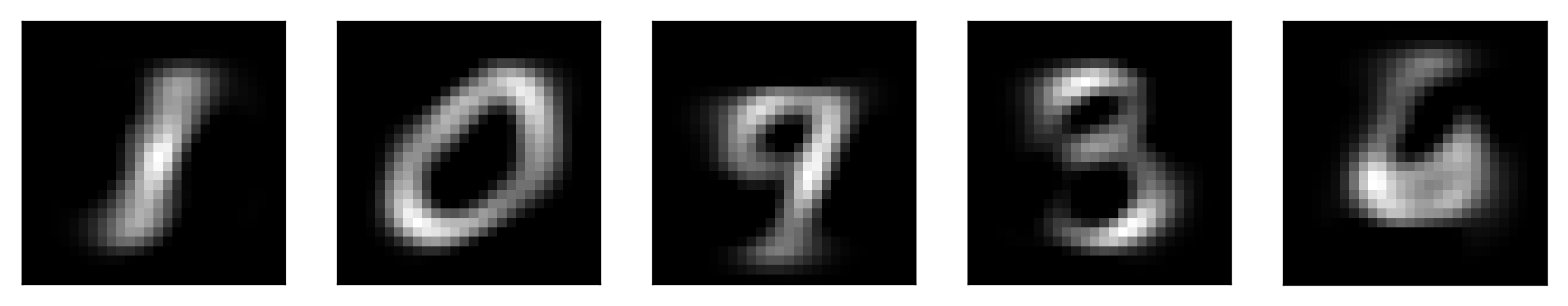
for ax, comp in zip(axes.ravel(), nmf5.components_):
ax.imshow(comp.reshape(28, 28), cmap="gray")
ax.set_xticks(())
ax.set_yticks(())
Outlier Detection
from sklearn.datasets import make_blobs
fig, ax = plt.subplots(1, 2, figsize=(6, 3))
X, y = make_blobs(random_state=1)
X_train, X_test, y_train, y_test = train_test_split(X, y, train_size=.9, random_state=0)
rng = np.random.RandomState(5)
X_train_noise = np.vstack([X_train, rng.uniform(X_train.min(), X_train.max(), size=(3, 2))])
y_train_noise = np.hstack([np.zeros_like(y_train), [1, 1, 1]])
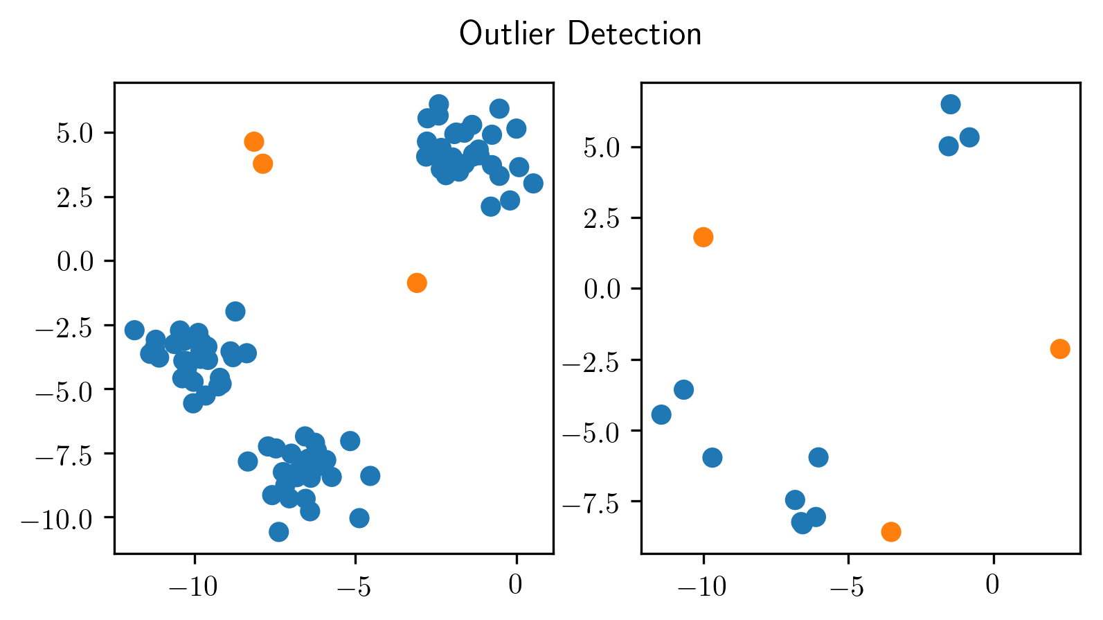
ax[0].scatter(X_train_noise[:, 0], X_train_noise[:, 1], c=plt.cm.Vega10(y_train_noise))
X_test_noise = np.vstack([X_test, rng.uniform(X_test.min(), X_test.max(), size=(4, 2))])
y_test_noise = np.hstack([np.zeros_like(y_test), [1, 0, 1, 1, 1]])
ax[1].scatter(X_test_noise[:, 0], X_test_noise[:, 1], c=plt.cm.Vega10(y_test_noise))
plt.suptitle("Outlier Detection")
<matplotlib.text.Text at 0x7fc8daef46d8>
from sklearn.datasets import make_blobs
fig, ax = plt.subplots(1, 2, figsize=(6, 3))
X, y = make_blobs(random_state=1)
X_train, X_test, y_train, y_test = train_test_split(X, y, train_size=.9, random_state=0)
rng = np.random.RandomState(5)
X_train_noise = np.vstack([X_train, rng.uniform(X_train.min(), X_train.max(), size=(3, 2))])
y_train_noise = np.hstack([np.zeros_like(y_train), [1, 1, 1]])
ax[0].scatter(X_train[:, 0], X_train[:, 1])
X_test_noise = np.vstack([X_test, rng.uniform(X_test.min(), X_test.max(), size=(4, 2))])
y_test_noise = np.hstack([np.zeros_like(y_test), [1, 0, 1, 1, 1]])
ax[1].scatter(X_test_noise[:, 0], X_test_noise[:, 1], c=plt.cm.Vega10(y_test_noise))
plt.suptitle("Novelty Detection")
<matplotlib.text.Text at 0x7fc8dad73cc0>
import numpy as np
import matplotlib.pyplot as plt

from sklearn.covariance import EmpiricalCovariance, MinCovDet

n_samples = 125
n_outliers = 25
n_features = 2

# generate data
gen_cov = np.eye(n_features)
gen_cov[0, 0] = 2.
X = np.dot(np.random.randn(n_samples, n_features), gen_cov)
# add some outliers
outliers_cov = np.eye(n_features)
outliers_cov[np.arange(1, n_features), np.arange(1, n_features)] = 7.
X[-n_outliers:] = np.dot(np.random.randn(n_outliers, n_features), outliers_cov)

# fit a Minimum Covariance Determinant (MCD) robust estimator to data
robust_cov = MinCovDet().fit(X)

# compare estimators learnt from the full data set with true parameters
emp_cov = EmpiricalCovariance().fit(X)

# Show data set
subfig1 = plt.gca()
inlier_plot = subfig1.scatter(X[:, 0], X[:, 1],
                              color='black', label='inliers')
outlier_plot = subfig1.scatter(X[:, 0][-n_outliers:], X[:, 1][-n_outliers:],
                               color='red', label='outliers')
subfig1.set_xlim(subfig1.get_xlim()[0], 11.)
subfig1.set_title("Mahalanobis distances of a contaminated data set:")

# Show contours of the distance functions
xx, yy = np.meshgrid(np.linspace(plt.xlim()[0], plt.xlim()[1], 100),
                     np.linspace(plt.ylim()[0], plt.ylim()[1], 100))
zz = np.c_[xx.ravel(), yy.ravel()]

mahal_emp_cov = emp_cov.mahalanobis(zz)
mahal_emp_cov = mahal_emp_cov.reshape(xx.shape)
emp_cov_contour = subfig1.contour(xx, yy, np.sqrt(mahal_emp_cov),
                                  cmap=plt.cm.PuBu_r,
                                  linestyles='dashed')

mahal_robust_cov = robust_cov.mahalanobis(zz)
mahal_robust_cov = mahal_robust_cov.reshape(xx.shape)
robust_contour = subfig1.contour(xx, yy, np.sqrt(mahal_robust_cov),
                                 cmap=plt.cm.YlOrBr_r, linestyles='dotted')

subfig1.legend([emp_cov_contour.collections[1], robust_contour.collections[1],
                inlier_plot, outlier_plot],
               ['MLE dist', 'robust dist', 'inliers', 'outliers'],
               loc="upper right", borderaxespad=0)
plt.xticks(())
plt.yticks(())
([], <a list of 0 Text yticklabel objects>)
from sklearn.covariance import EllipticEnvelope
ee = EllipticEnvelope(contamination=.1).fit(X)
pred = ee.predict(X)
print(pred)
print(np.mean(pred == -1))
[ 1  1  1  1  1  1  1  1  1  1  1  1  1  1  1  1  1  1  1  1  1  1  1  1  1
  1  1  1  1  1  1  1  1  1  1  1  1  1  1  1  1  1  1  1  1  1  1  1  1  1
  1  1  1  1  1  1  1  1  1  1  1  1  1  1  1  1  1  1  1  1  1  1  1  1  1
  1  1  1  1  1  1  1  1  1  1  1  1  1  1  1  1  1  1  1  1  1  1  1  1  1
 -1  1  1  1 -1 -1  1 -1  1  1 -1  1 -1 -1 -1  1  1 -1 -1 -1 -1  1 -1  1  1]
0.104
from sklearn.covariance import EllipticEnvelope
ee = EllipticEnvelope(contamination=.1).fit(X_train_noise)
pred = ee.predict(X_train_noise)
plt.scatter(X_train_noise[:, 0], X_train_noise[:, 1], c=plt.cm.Vega10(pred))
<matplotlib.collections.PathCollection at 0x7fc8da8fe198>
from sklearn.neighbors import KernelDensity
kde = KernelDensity().fit(X_noise[:, :1])

line = np.linspace(X_noise.min(), 3, 100)
line_density = kde.score_samples(line[:, np.newaxis])

plt.plot(line, line_density)
plt.plot(X_noise[:, 0], -5 * np.ones(X_noise.shape[0]), 'o')
plt.ylim(-6, -2)
(-6, -2)
kde = KernelDensity(bandwidth=.3).fit(X_noise[:, :1])

line = np.linspace(X_noise.min(), 3, 100)
line_density = kde.score_samples(line[:, np.newaxis])

plt.plot(line, line_density)
plt.plot(X_noise[:, 0], -5 * np.ones(X_noise.shape[0]), 'o')
plt.ylim(-7, 1)
(-7, 1)
kde = KernelDensity(bandwidth=3)
kde.fit(X_train_noise)
pred = kde.score_samples(X_train_noise)
pred = (pred > np.percentile(pred, 10)).astype(int)
xs = np.linspace(xlim[0], xlim[1], 100)
ys = np.linspace(ylim[0], ylim[1], 100)
xx, yy = np.meshgrid(xs, ys)
dec = kde.score_samples(np.c_[xx.ravel(), yy.ravel()])

plt.xlim(xlim)
plt.ylim(ylim)
plt.contourf(xx, yy, dec.reshape(xx.shape), alpha=.5)
pred = kde.score_samples(X_train_noise)
pred = (pred > np.percentile(pred, 10)).astype(int)
plt.scatter(X_train_noise[:, 0], X_train_noise[:, 1], c=plt.cm.Vega10(pred))
<matplotlib.collections.PathCollection at 0x7fc8d8ed5a90>
from sklearn.svm import OneClassSVM
scaler = StandardScaler()
X_train_noise_scaled = scaler.fit_transform(X_train_noise)
oneclass = OneClassSVM(nu=.1).fit(X_train_noise_scaled)
pred = oneclass.predict(X_train_noise_scaled).astype(np.int)
dec = oneclass.decision_function(scaler.transform(np.c_[xx.ravel(), yy.ravel()]))
plt.xlim(xlim)
plt.ylim(ylim)
plt.contourf(xx, yy, dec.reshape(xx.shape), alpha=.5)
plt.scatter(X_train_noise[:, 0], X_train_noise[:, 1], c=plt.cm.Vega10(pred))
<matplotlib.collections.PathCollection at 0x7fc8d89f5e48>
from sklearn.ensemble import IsolationForest
iso = IsolationForest().fit(X_train_noise)
pred = iso.predict(X_train_noise)
plt.scatter(X_train_noise[:, 0], X_train_noise[:, 1], c=plt.cm.Vega10(pred))
xlim = plt.xlim()
ylim = plt.ylim()
xs = np.linspace(xlim[0], xlim[1], 100)
ys = np.linspace(ylim[0], ylim[1], 100)
xx, yy = np.meshgrid(xs, ys)
dec = iso.decision_function(np.c_[xx.ravel(), yy.ravel()])
plt.xlim(xlim)
plt.ylim(ylim)
plt.contourf(xx, yy, dec.reshape(xx.shape), alpha=.5)
plt.scatter(X_train_noise[:, 0], X_train_noise[:, 1], c=plt.cm.Vega10(pred))
<matplotlib.collections.PathCollection at 0x7fc8d9456128>
data = pd.read_csv("creditcard.csv")
data.shape
(284807, 31)
data.head()
| Time | V1 | V2 | V3 | V4 | V5 | V6 | V7 | V8 | V9 | ... | V21 | V22 | V23 | V24 | V25 | V26 | V27 | V28 | Amount | Class | |
|---|---|---|---|---|---|---|---|---|---|---|---|---|---|---|---|---|---|---|---|---|---|
| 0 | 0.0 | -1.359807 | -0.072781 | 2.536347 | 1.378155 | -0.338321 | 0.462388 | 0.239599 | 0.098698 | 0.363787 | ... | -0.018307 | 0.277838 | -0.110474 | 0.066928 | 0.128539 | -0.189115 | 0.133558 | -0.021053 | 149.62 | 0 |
| 1 | 0.0 | 1.191857 | 0.266151 | 0.166480 | 0.448154 | 0.060018 | -0.082361 | -0.078803 | 0.085102 | -0.255425 | ... | -0.225775 | -0.638672 | 0.101288 | -0.339846 | 0.167170 | 0.125895 | -0.008983 | 0.014724 | 2.69 | 0 |
| 2 | 1.0 | -1.358354 | -1.340163 | 1.773209 | 0.379780 | -0.503198 | 1.800499 | 0.791461 | 0.247676 | -1.514654 | ... | 0.247998 | 0.771679 | 0.909412 | -0.689281 | -0.327642 | -0.139097 | -0.055353 | -0.059752 | 378.66 | 0 |
| 3 | 1.0 | -0.966272 | -0.185226 | 1.792993 | -0.863291 | -0.010309 | 1.247203 | 0.237609 | 0.377436 | -1.387024 | ... | -0.108300 | 0.005274 | -0.190321 | -1.175575 | 0.647376 | -0.221929 | 0.062723 | 0.061458 | 123.50 | 0 |
| 4 | 2.0 | -1.158233 | 0.877737 | 1.548718 | 0.403034 | -0.407193 | 0.095921 | 0.592941 | -0.270533 | 0.817739 | ... | -0.009431 | 0.798278 | -0.137458 | 0.141267 | -0.206010 | 0.502292 | 0.219422 | 0.215153 | 69.99 | 0 |
5 rows × 31 columns
X_train, X_test, y_train, y_test = train_test_split(data.drop("Class", axis=1), data.Class, train_size=.1, random_state=0)
X_train.shape
(28480, 30)
scaler = StandardScaler()
X_train_scaled = scaler.fit_transform(X_train)
ee = EllipticEnvelope().fit(X_train_scaled)
# => error
---------------------------------------------------------------------------
ValueError                                Traceback (most recent call last)
<ipython-input-240-efde2cb2e7b3> in <module>()
----> 1 ee = EllipticEnvelope().fit(X_train_scaled)
      2 # => error

/home/andy/checkout/scikit-learn/sklearn/covariance/outlier_detection.py in fit(self, X, y)
    173
    174     def fit(self, X, y=None):
--> 175         MinCovDet.fit(self, X)
    176         self.threshold_ = sp.stats.scoreatpercentile(
    177             self.dist_, 100. * (1. - self.contamination))

/home/andy/checkout/scikit-learn/sklearn/covariance/robust_covariance.py in fit(self, X, y)
    617             X, support_fraction=self.support_fraction,
    618             cov_computation_method=self._nonrobust_covariance,
--> 619             random_state=random_state)
    620         if self.assume_centered:
    621             raw_location = np.zeros(n_features)

/home/andy/checkout/scikit-learn/sklearn/covariance/robust_covariance.py in fast_mcd(X, support_fraction, cov_computation_method, random_state)
    433                 select=n_best_sub, n_iter=2,
    434                 cov_computation_method=cov_computation_method,
--> 435                 random_state=random_state)
    436             subset_slice = np.arange(i * n_best_sub, (i + 1) * n_best_sub)
    437             all_best_locations[subset_slice] = best_locations_sub

/home/andy/checkout/scikit-learn/sklearn/covariance/robust_covariance.py in select_candidates(X, n_support, n_trials, select, n_iter, verbose, cov_computation_method, random_state)
    272                     X, n_support, remaining_iterations=n_iter, verbose=verbose,
    273                     cov_computation_method=cov_computation_method,
--> 274                     random_state=random_state))
    275     else:
    276         # perform computations from every given initial estimates

/home/andy/checkout/scikit-learn/sklearn/covariance/robust_covariance.py in _c_step(X, n_support, random_state, remaining_iterations, initial_estimates, verbose, cov_computation_method)
    144     if np.isinf(det):
    145         raise ValueError(
--> 146             "Singular covariance matrix. "
    147             "Please check that the covariance matrix corresponding "
    148             "to the dataset is full rank and that MinCovDet is used with "

ValueError: Singular covariance matrix. Please check that the covariance matrix corresponding to the dataset is full rank and that MinCovDet is used with Gaussian-distributed data (or at least data drawn from a unimodal, symmetric distribution.
from sklearn.decomposition import PCA
X_train_pca = PCA(n_components=.8).fit_transform(X_train_scaled)
ee = EllipticEnvelope().fit(X_train_pca)
from sklearn.metrics import roc_auc_score
roc_auc_score(y_train, ee.mahalanobis(X_train_pca))
0.91699652177871382