Data Splitting Strategies
Do importance of pipelines here?
Cross-Validation Strategies
So I mentioned k-fold cross validation, where k is usually 5 or ten, but there are many other strategies.
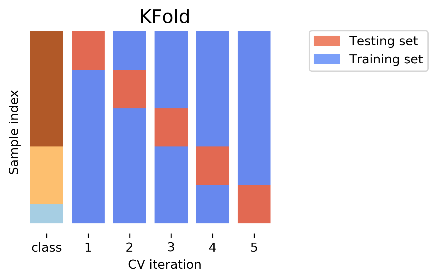
One of the most commonly ones is stratified k-fold cross-validation.
.center[
 ]
]
.center[
 ]
.smallest[
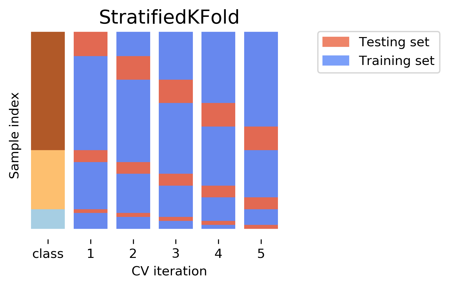
Stratified:
Ensure relative class frequencies in each fold reflect relative class
frequencies on the whole dataset.]
The idea behind stratified k-fold cross-validation is that you want the test set to be as representative of the dataset as possible. StratifiedKFold preserves the class frequencies in each fold to be the same as of the overall dataset. Here is and example of a dataset with three classes that are ordered. If you apply standard three-fold to this, the first third of the data would be in the first fold, the second in the second fold and the third in the third fold. Because this data is sorted, that would be particularly bad. If you use stratified cross-validation it would make sure that each fold has exactly 1/3 of the data from each class.
This is also helpful if your data is very imbalanced. If some of the classes are very rare, it could otherwise happen that a class is not present at all in a particular fold.
Importance of Stratification
.smaller[
y.value_counts()
0    60
1    40
from sklearn.model_selection import cross_val_score, KFold, StratifiedKFold
from sklearn.dummy import DummyClassifier

dc = DummyClassifier('most_frequent')
skf = StratifiedKFold(n_splits=5, shuffle=True)
res = cross_val_score(dc, X, y, cv=skf)
np.mean(res), res.std()
(0.6, 0.0)
kf = KFold(n_splits=5, shuffle=True)
res = cross_val_score(dc, X, y, cv=kf)
np.mean(res), res.std()
(0.6, 0.063)
]
Repeated KFold and LeaveOneOut
LeaveOneOut : KFold(n_folds=n_samples)
High variance, takes a long time
.tiny[(see Raschka for a review and Varoquaux for empirical evaluation)]
Better: ShuffleSplit (aka Monte Carlo)
Repeatedly sample a test set with replacement
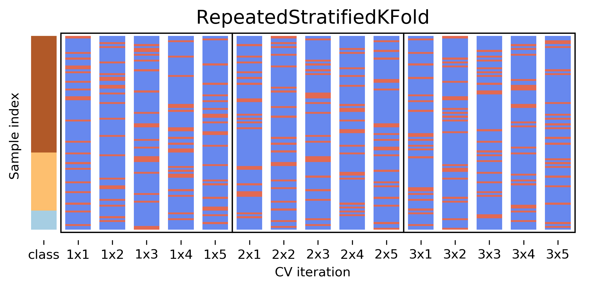
Even Better: RepeatedKFold.
Apply KFold or StratifiedKFold multiple times with shuffled data.
If you want even better estimates of the generalization performance, you could try to increase the number of folds, with the extreme of creating one fold per sample. That’s called “LeaveOneOut cross-validation”. However, because the test-set is so small every time, and the training sets all have very large overlap, this method has very high variance. A better way to get a robust estimate is to run 5-fold or 10-fold cross-validation multiple times, while shuffling the dataset.
.center[
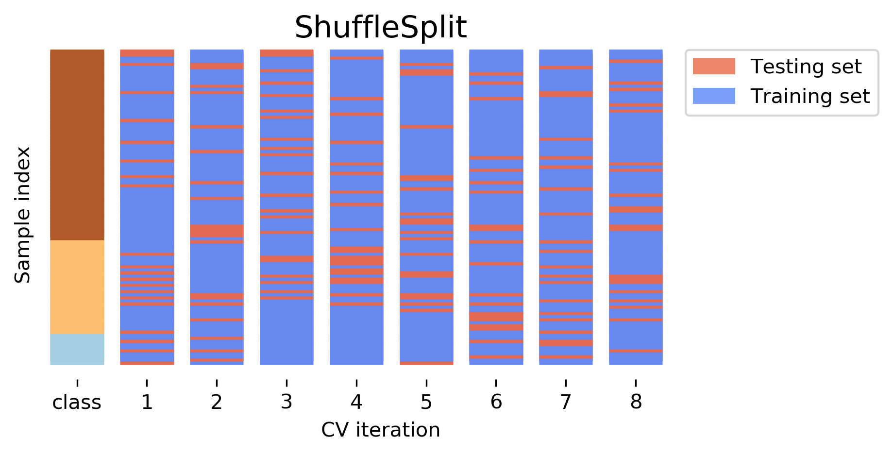 ]
.smaller[Number of iterations and test set size independent]
Another interesting variant is shuffle split and stratified shuffle split. In shuffle split, we repeatedly sample disjoint training and test sets randomly. You only have to specify the number of iterations, the training set size and the test set size. This also allows you to run many iterations with reasonably large test-sets. It’s also great if you have a very large training set and you want to subsample it to get quicker results.
.center[
 ]
.smaller[
Potentially less variance than StratifiedShuffleSplit.
Five times five fold or at most ten times ten fold is sufficient. ]
Defaults in scikit-learn
5-fold in 0.22 (used to be 3 fold)
For classification cross-validation is stratified
train_test_split has stratify option: train_test_split(X, y, stratify=y)
No shuffle by default!
By default, all cross-validation strategies are five fold. If you do cross-validation for classification, it will be stratified by default. Because of how the interface is done, that’s not true for train_test_split and if you want a stratified train_test_split, which is always a good idea, you should use stratify=y Another thing that’s important to keep in mind is that by default scikit-learn doesn’t shuffle! So if you run cross-validation twice with the default parameters, it will yield exactly the same results.
Cross-Validation with non-iid data
Grouped Data
Assume have data (medical, product, user…) from 5 cities
New York, San Francisco, Los Angeles, Chicago, Houston.
We can assume data within a city is more correlated then between cities.
Usage Scenarios
Assume all future users will be in one of these cities: i.i.d.
Assume we want to generalize to predict for a new city: not i.i.d.
Shipped product in 4 cities. Might ship in another one? States: you have all the states, no new state will start to exist
Similar thing for multiple measurements per patient. Or geospacial data.
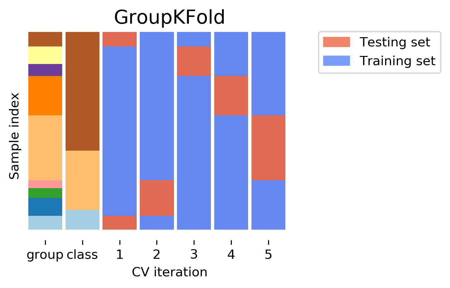
A somewhat more complicated approach is group k-fold. This is actually for data that doesn’t fulfill our IID assumption and has correlations between samples. The idea is that there are several groups in the data that each contain highly correlated samples. You could think about patient data where you have multiple samples for each patient, then the groups would be which patient a measurement was taken from. If you want to know how well your model generalizes to new patients, you need to ensure that the measurements from each patient are either all in the training set, or all in the test set. And that’s what GroupKFold does. In this example, there are four groups, and we want three folds. The data is divided such that each group is contained in exactly one fold. There are several other cross-validation methods in scikit-learn that use these groups.
Correlations in time (and/or space)
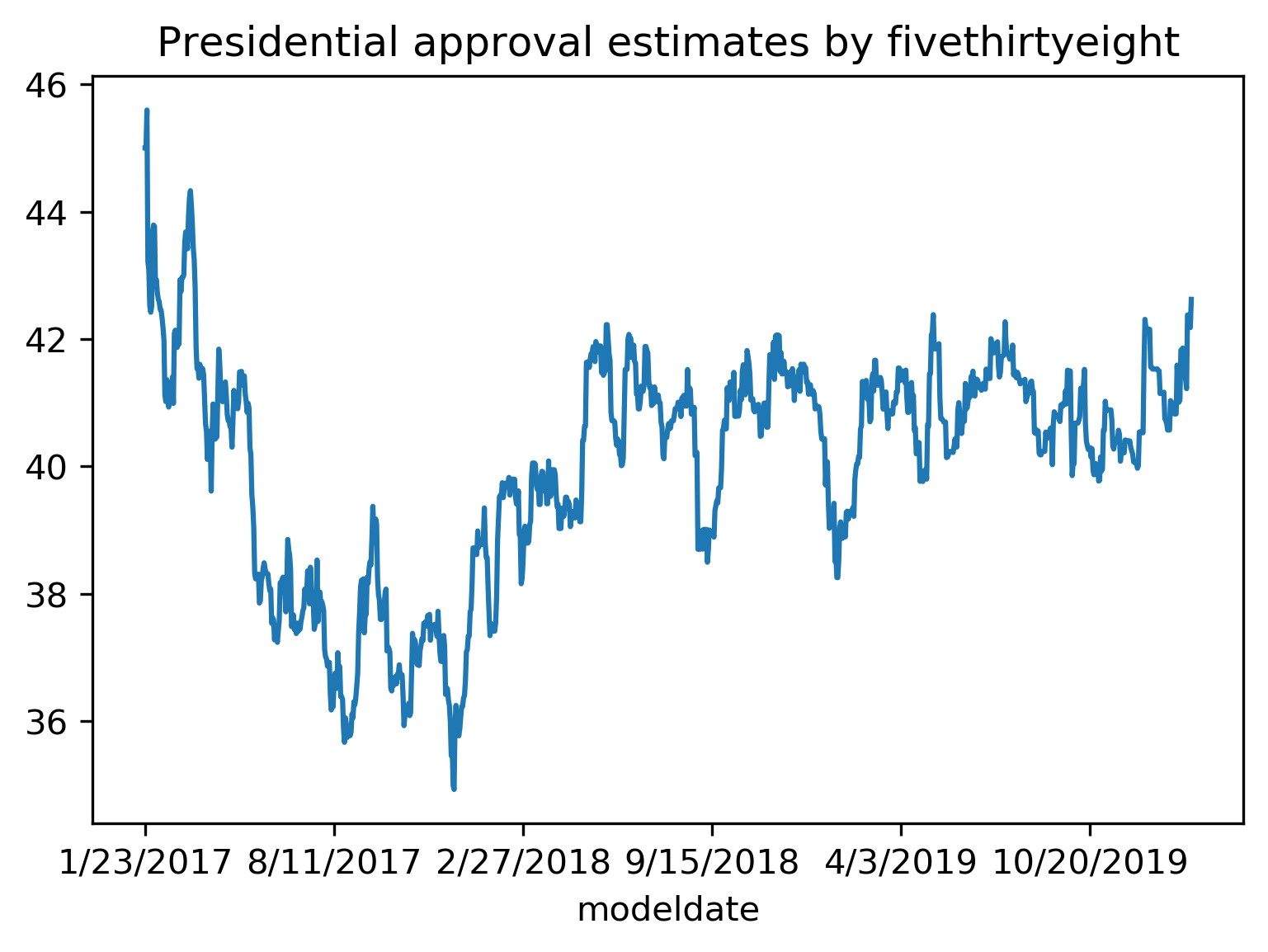
Not necessarily obvious that there is a time component! Data collection usually happens over time!
Correlations in time (and/or space)
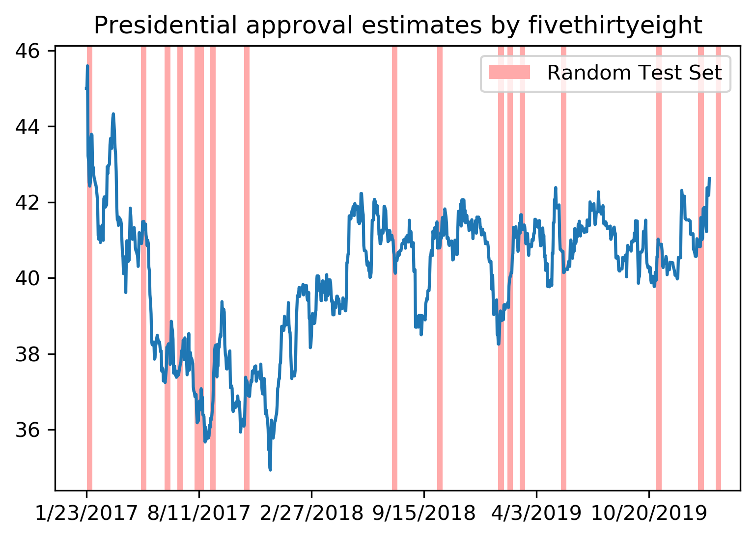
Not necessarily obvious that there is a time component! Data collection usually happens over time!
Correlations in time (and/or space)
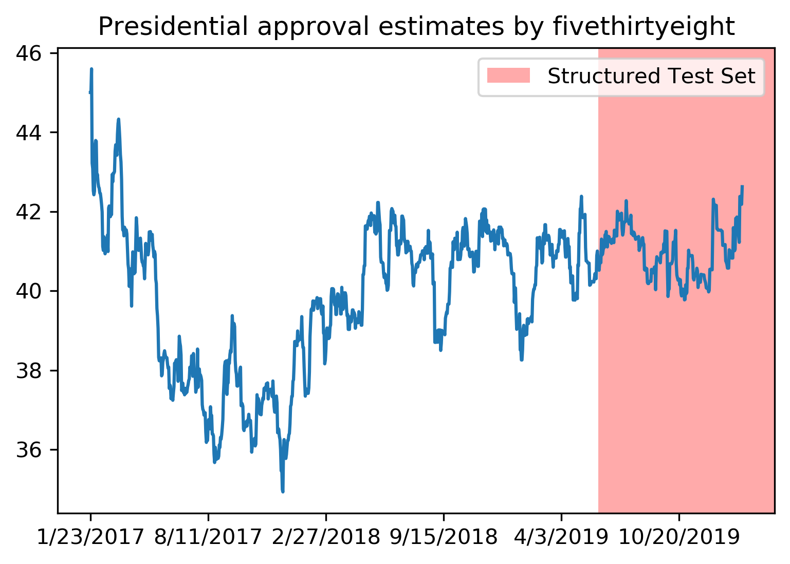
Not necessarily obvious that there is a time component! Data collection usually happens over time!
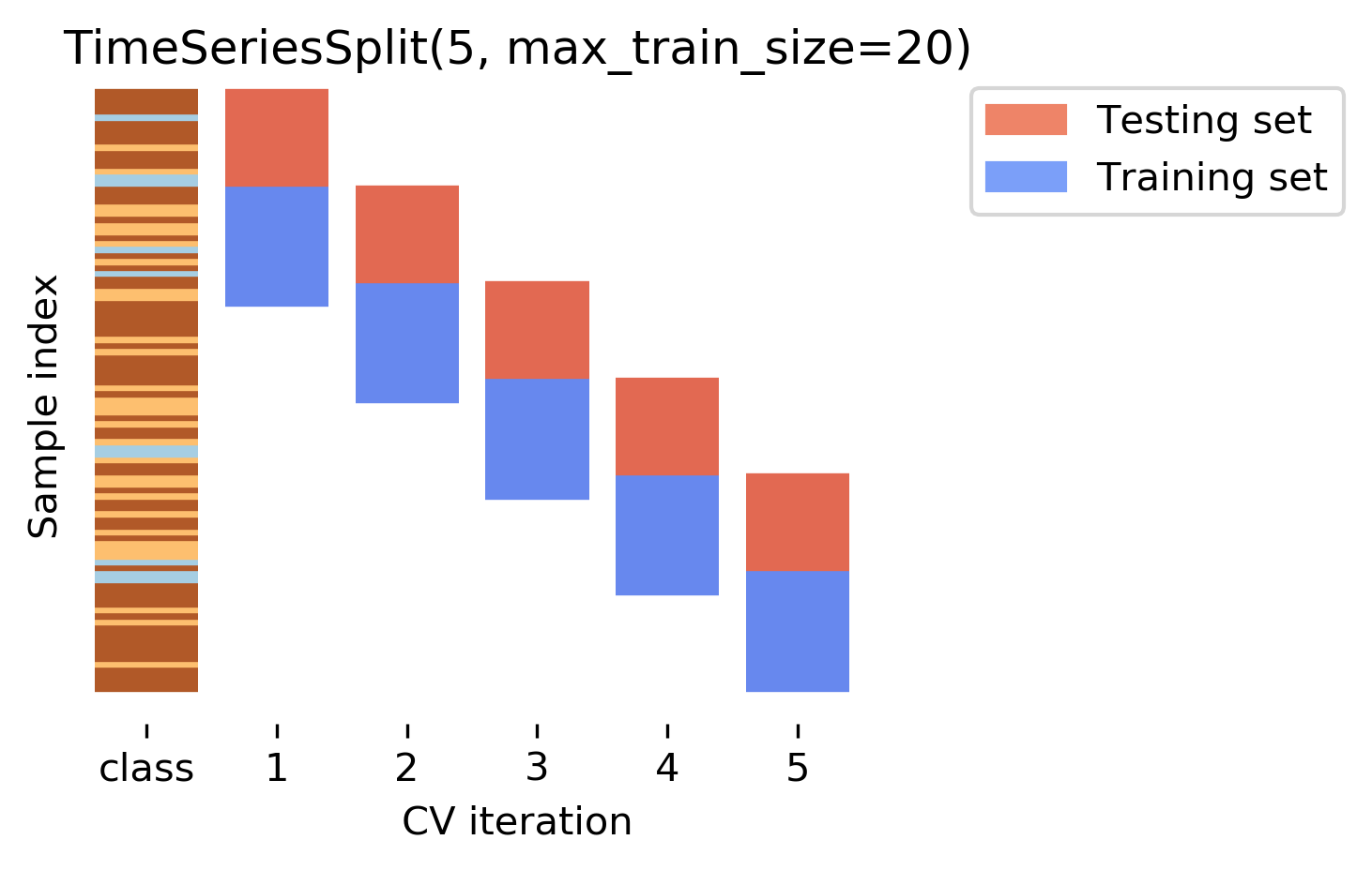
Another common case of data that’s not independent is time series. Usually todays stock price is correlated with yesterdays and tomorrows. If you randomly split time series, this makes predictions deceivingly simple. In applications, you usually have data up to some point, and then try to make predictions for the future, in other words, you’re trying to make a forecast. The TimeSeriesSplit in scikit-learn simulates that, by taking increasing chunks of data from the past and making predictions on the next chunk. This is quite different from the other was to do cross-validation, in that the training sets are all overlapping, but it’s more appropriate for time-series.
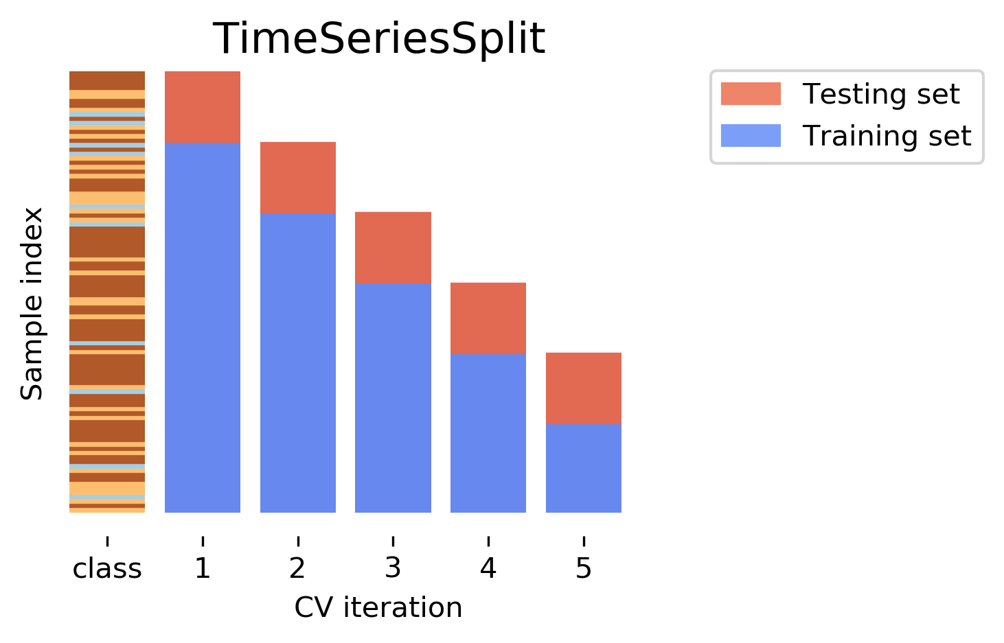
Another common case of data that’s not independent is time series. Usually todays stock price is correlated with yesterdays and tomorrows. If you randomly split time series, this makes predictions deceivingly simple. In applications, you usually have data up to some point, and then try to make predictions for the future, in other words, you’re trying to make a forecast. The TimeSeriesSplit in scikit-learn simulates that, by taking increasing chunks of data from the past and making predictions on the next chunk. This is quite different from the other was to do cross-validation, in that the training sets are all overlapping, but it’s more appropriate for time-series.
Using Cross-Validation Generators
.tiny[
from sklearn.model_selection import KFold, StratifiedKFold, ShuffleSplit, RepeatedStratifiedKFold
kfold = KFold(n_splits=5)
skfold = StratifiedKFold(n_splits=5, shuffle=True)
ss = ShuffleSplit(n_splits=20, train_size=.4, test_size=.3)
rs = RepeatedStratifiedKFold(n_splits=5, n_repeats=10)

print("KFold:")
print(cross_val_score(KNeighborsClassifier(), X, y, cv=kfold))

print("StratifiedKFold:")
print(cross_val_score(KNeighborsClassifier(), X, y, cv=skfold))

print("ShuffleSplit:")
print(cross_val_score(KNeighborsClassifier(), X, y, cv=ss))

print("RepeatedStratifiedKFold:")
print(cross_val_score(KNeighborsClassifier(), X, y, cv=rs))
KFold:
[0.93 0.96 0.96 0.98 0.96]
StratifiedKFold:
[0.98 0.96 0.96 0.97 0.96]
ShuffleSplit:
[0.98 0.96 0.96 0.98 0.94 0.96 0.95 0.98 0.97 0.92 0.94 0.97 0.95 0.92
 0.98 0.98 0.97 0.94 0.97 0.95]
RepeatedStratifiedKFold:
[0.99 0.96 0.97 0.97 0.95 0.98 0.97 0.98 0.97 0.96 0.97 0.99 0.94 0.96
 0.96 0.98 0.97 0.96 0.96 0.97 0.97 0.96 0.96 0.96 0.98 0.96 0.97 0.97
 0.97 0.96 0.96 0.95 0.96 0.99 0.98 0.93 0.96 0.98 0.98 0.96 0.96 0.95
 0.97 0.97 0.96 0.97 0.97 0.97 0.96 0.96]
]
Ok, so how do we use these cross-validation generators? We can simply pass the object to the cv parameter of the cross_val_score function, instead of passing a number. Then that generator will be used. Here are some examples for k-neighbors classifier. We instantiate a Kfold object with the number of splits equal to 5, and then pass it to cross_val_score. We can do the same with StratifiedKFold, and we can also shuffle if we like, or we can use Shuffle split.
cross_validate function
.smaller[
from sklearn.model_selection import cross_validate
res = cross_validate(KNeighborsClassifier(), X, y, return_train_score=True,
                     scoring=["accuracy", "roc_auc"])
res_df = pd.DataFrame(res)
fit_time	score_time	test_accuracy	test_roc_auc	train_accuracy	train_roc_auc
0.000839	0.010204    0.965217	    0.996609	    0.980176	    0.997654
0.000870	0.014424    0.956522	    0.983689	    0.975771	    0.998650
0.000603	0.009298    0.982301	    0.999329	    0.971491	    0.996977
0.000698	0.006670    0.955752	    0.984071	    0.978070	    0.997820
0.000611	0.006559    0.964602	    0.994634	    0.978070	    0.998026
]
FIXME alignment
Questions ?
import matplotlib.pyplot as plt
import numpy as np
import sklearn
sklearn.set_config(print_changed_only=True)
from sklearn.datasets import load_digits
from sklearn.model_selection import train_test_split

digits = load_digits()
X_train, X_test, y_train, y_test = train_test_split(
    digits.data, digits.target)
from sklearn.model_selection import cross_val_score
from sklearn.neighbors import KNeighborsClassifier
cross_val_score(KNeighborsClassifier(),
                X_train, y_train, cv=5)
from sklearn.model_selection import KFold, RepeatedStratifiedKFold
cross_val_score(KNeighborsClassifier(),
                X_train, y_train, cv=KFold(n_splits=10, shuffle=True, random_state=42))
cross_val_score(KNeighborsClassifier(),
                X_train, y_train,
                cv=RepeatedStratifiedKFold(n_splits=10, n_repeats=10, random_state=42))
Grid Searches
Grid-Search with build-in cross validation
from sklearn.model_selection import GridSearchCV
from sklearn.svm import SVC
Define parameter grid:
import numpy as np

param_grid = {'C': 10. ** np.arange(-3, 3),
              'gamma' : 10. ** np.arange(-5, 0)}

np.set_printoptions(suppress=True)
print(param_grid)
grid_search = GridSearchCV(SVC(), param_grid, verbose=3)
A GridSearchCV object behaves just like a normal classifier.
grid_search.fit(X_train, y_train)
grid_search.predict(X_test)
grid_search.score(X_test, y_test)
grid_search.best_params_
grid_search.best_score_
grid_search.best_estimator_
# We extract just the scores

scores = grid_search.cv_results_['mean_test_score']
scores = np.array(scores).reshape(6, 5)

plt.matshow(scores)
plt.xlabel('gamma')
plt.ylabel('C')
plt.colorbar()
plt.xticks(np.arange(5), param_grid['gamma'])
plt.yticks(np.arange(6), param_grid['C']);
Exercises
Use GridSearchCV to adjust n_neighbors of KNeighborsClassifier.
Model complexity
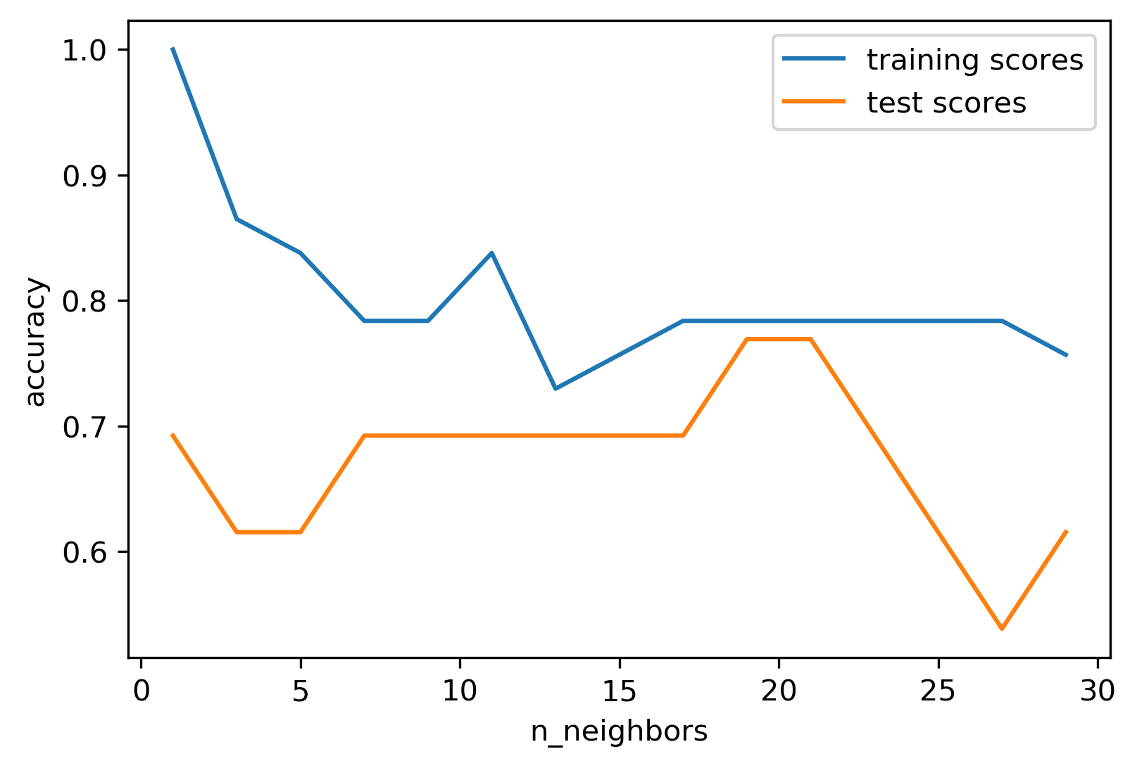
We can look at this in more detail by comparing training and test set scores for the different numbers of neighbors. Here, I did a random 75%/25% split again. This is a very noisy plot as the dataset is very small and I only did a random split, but you can see a trend here. You can see that for a single neighbor, the training score is 1 so perfect accuracy, but the test score is only 70%. If we increase the number of neighbors we consider, the training score goes down, but the test score goes up, with an optimum at 19 and 21, but then both go down again.
This is a very typical behavior, that I sketched in a schematic for you.
here is a cartoon version of how this chart looks in general, though it’s horizontally flipped to the one with saw for knn. This chart has accuracy on the y axis, and the abstract concept of model complexity on the x axis. If we make our machine learning models more complex, we will get better training set accuracy, as the model will be able to capture more of the variations in the data.
But if we look at the generalization performance, we get a different story. If the model complexity is too low, the model will not be able to capture the main trends, and a more complex model means better generalization. However, if we make the model too complex, generalization performance drops again, because we basically learn to memorize the dataset.
Overfitting and Underfitting
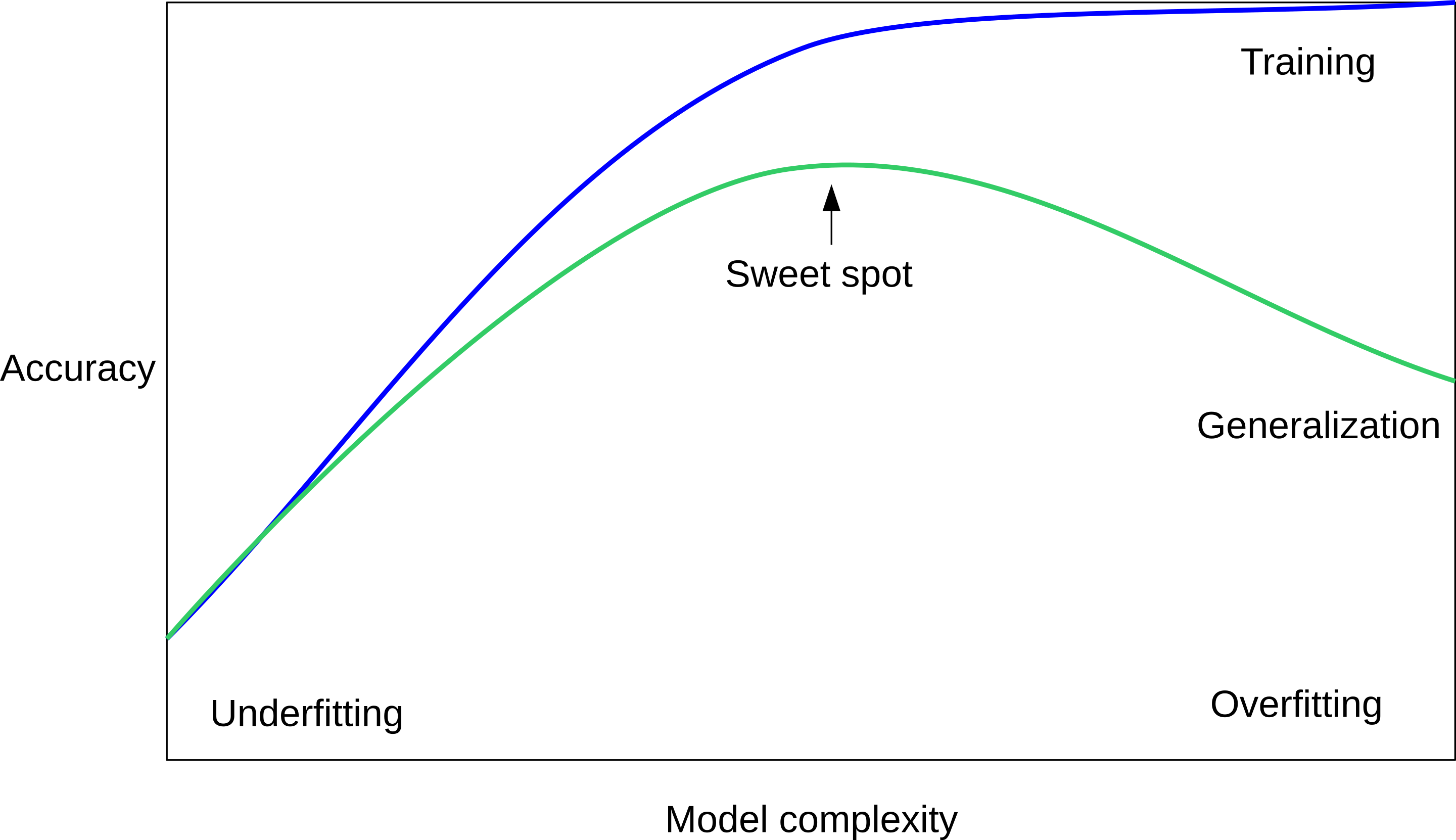
If we use too simple a model, this is often called underfitting, while if we use to complex a model, this is called overfitting. And somewhere in the middle is a sweet spot. Most models have some way to tune model complexity, and we’ll see many of them in the next couple of weeks. So going back to nearest neighbors, what parameters correspond to high model complexity and what to low model complexity? high n_neighbors = low complexity!
# %load solutions/grid_search_k_neighbors.py
Not using Pipelines vs feature selection
rnd = np.random.RandomState(seed=0)
X = rnd.normal(size=(100, 10000))
X_test = rnd.normal(size=(100, 10000))
y = rnd.normal(size=(100,))
y_test = rnd.normal(size=(100,))
from sklearn.feature_selection import SelectPercentile, f_regression

select = SelectPercentile(score_func=f_regression,
                          percentile=5)
select.fit(X, y)
X_selected = select.transform(X)
print(X_selected.shape)
from sklearn.model_selection import cross_val_score
from sklearn.linear_model import Ridge
np.mean(cross_val_score(Ridge(), X_selected, y))
ridge = Ridge().fit(X_selected, y)
X_test_selected = select.transform(X_test)
ridge.score(X_test_selected, y_test)
Back to house price?
from sklearn.linear_model import Ridge
X, y = df, target
X_train, X_test, y_train, y_test = train_test_split(X, y, random_state=0)

scaler = StandardScaler()
scaler.fit(X_train)
X_train_scaled = scaler.transform(X_train)
ridge = Ridge().fit(X_train_scaled, y_train)

X_test_scaled = scaler.transform(X_test)
ridge.score(X_test_scaled, y_test)
from sklearn.pipeline import make_pipeline
pipe = make_pipeline(StandardScaler(), Ridge())
pipe.fit(X_train, y_train)
pipe.score(X_test, y_test)
rnd = np.random.RandomState(seed=0)
X = rnd.normal(size=(100, 10000))
X_test = rnd.normal(size=(100, 10000))
y = rnd.normal(size=(100,))
y_test = rnd.normal(size=(100,))
from sklearn.pipeline import Pipeline

pipe = Pipeline([("select", select),
                 ("ridge", Ridge())])
np.mean(cross_val_score(pipe, X, y))
from sklearn.linear_model import Ridge
X, y = df, target
X_train, X_test, y_train, y_test = train_test_split(X, y, random_state=0)
from sklearn.pipeline import Pipeline
pipe = Pipeline((("scaler", StandardScaler()),
                 ("regressor", KNeighborsRegressor)))
from sklearn.model_selection import GridSearchCV

knn_pipe = make_pipeline(StandardScaler(), KNeighborsRegressor())
param_grid = {'kneighborsregressor__n_neighbors': range(1, 10)}
grid = GridSearchCV(knn_pipe, param_grid, cv=10)
grid.fit(X_train, y_train)
print(grid.best_params_)
print(grid.score(X_test, y_test))
from sklearn.datasets import load_diabetes
diabetes = load_diabetes()
X_train, X_test, y_train, y_test = train_test_split(
    diabetes.data, diabetes.target, random_state=0)

from sklearn.preprocessing import PolynomialFeatures
pipe = make_pipeline(
    StandardScaler(),
    PolynomialFeatures(),
    Ridge())
param_grid = {'polynomialfeatures__degree': [1, 2, 3],
              'ridge__alpha': [0.001, 0.01, 0.1, 1, 10, 100]}
grid = GridSearchCV(pipe, param_grid=param_grid,
                    n_jobs=-1, return_train_score=True)
grid.fit(X_train, y_train)
from sklearn.linear_model import Lasso

pipe = Pipeline([('scaler', StandardScaler()), ('regressor', Ridge())])

param_grid = {'scaler': [StandardScaler(), MinMaxScaler(), 'passthrough'],
              'regressor': [Ridge(), Lasso()],
              'regressor__alpha': np.logspace(-3, 3, 7)}


grid = GridSearchCV(pipe, param_grid)
grid.fit(X_train, y_train)
grid.score(X_test, y_test)
from sklearn.tree import DecisionTreeRegressor
pipe = Pipeline([('scaler', StandardScaler()), ('regressor', Ridge())])

param_grid = [{'regressor': [DecisionTreeRegressor()],
               'regressor__max_depth': [2, 3, 4],
               'scaler': ['passthrough']},
              {'regressor': [Ridge()],
               'regressor__alpha': [0.1, 1],
               'scaler': [StandardScaler(), MinMaxScaler(), 'passthrough']}
             ]
grid = GridSearchCV(pipe, param_grid)
grid.fit(X_train, y_train)
grid.score(X_test, y_test)
0.36901969445308325
