Feature Engineering
interesting random states
18 0.486666666667 0.986666666667 42 0.553333333333 0.986666666667 44 0.526666666667 1.0 54 0.56 1.0 67 0.506666666667 1.0 70 0.586666666667 1.0 79 0.673333333333 1.0 96 0.526666666667 1.0 161 0.486666666667 1.0 174 0.566666666667 1.0 175 0.62 1.0
from sklearn.datasets import make_blobs
from sklearn.preprocessing import scale
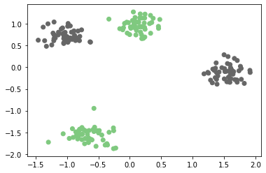
X, y = make_blobs(n_samples=200, centers=4, random_state=42)
X = scale(X)
y = y % 2
plt.scatter(X[:, 0], X[:, 1], c=y, cmap='Accent')
<matplotlib.collections.PathCollection at 0x7f4bdff125c0>
from sklearn.linear_model import LogisticRegressionCV
X_train, X_test, y_train, y_test = train_test_split(X, y, random_state=0)
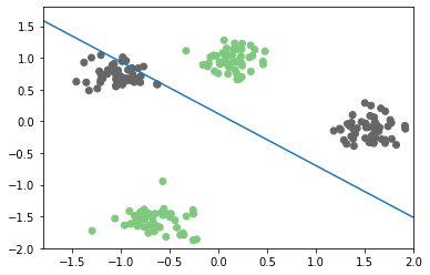
logreg = LogisticRegressionCV().fit(X_train, y_train)
logreg.score(X_test, y_test)
0.5
plt.scatter(X[:, 0], X[:, 1], c=y, cmap='Accent')
line = np.linspace(-3, 3, 100)
coef = logreg.coef_.ravel()

plt.plot(line, -(coef[0] * line + logreg.intercept_) / coef[1])

plt.xlim(-1.8, 2)
plt.ylim(-2, 1.8)
(-2, 1.8)
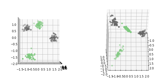
# Same as PolynomialFeatures(order=2, interactions_only=True)
X_interaction = np.hstack([X, X[:, 0:1] * X[:, 1:]])
from mpl_toolkits.mplot3d import Axes3D
fig = plt.figure(figsize=(10, 5))
ax = fig.add_subplot(121, projection='3d')
ax.scatter(X_interaction[:, 2], X_interaction[:, 0], X_interaction[:, 1], c=y, cmap="Accent")
ax.view_init(elev=0., azim=0)

ax = fig.add_subplot(122, projection='3d')
ax.scatter(X_interaction[:, 2], X_interaction[:, 0], X_interaction[:, 1], c=y, cmap="Accent")
ax.view_init(elev=60., azim=0)
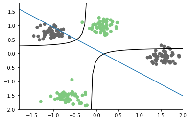
X_i_train, X_i_test, y_train, y_test = train_test_split(X_interaction, y, random_state=0)
logreg3 = LogisticRegressionCV().fit(X_i_train, y_train)
logreg3.score(X_i_test, y_test)
0.96
plt.scatter(X[:, 0], X[:, 1], c=y, cmap='Accent')
line = np.linspace(-3, 3, 100)
coef = logreg.coef_.ravel()
coef3 = logreg3.coef_.ravel()
plt.plot(line, -(coef[0] * line + logreg.intercept_) / coef[1])
curve = -(coef3[0] * line + logreg3.intercept_) / (coef3[1] + line * coef3[2])
mask = coef3[1] + line * coef3[2] > 0
plt.plot(line[mask], curve[mask], c='k')
plt.plot(line[~mask], curve[~mask], c='k')
plt.xlim(-1.8, 2)
plt.ylim(-2, 1.8)
(-2, 1.8)
Discrete interactions
df = pd.DataFrame({'gender': ['M', 'F', 'M', 'F', 'F'],
                   'age': [14, 16, 12, 25, 22],
                   'spend$': [70, 12, 42, 64, 93],
                   'articles_bought': [5, 10, 2, 1, 1],
                   'time_online': [269, 1522, 235, 63, 21]
                  })
df
| gender | age | spend$ | articles_bought | time_online | |
|---|---|---|---|---|---|
| 0 | M | 14 | 70 | 5 | 269 |
| 1 | F | 16 | 12 | 10 | 1522 |
| 2 | M | 12 | 42 | 2 | 235 |
| 3 | F | 25 | 64 | 1 | 63 |
| 4 | F | 22 | 93 | 1 | 21 |
dummies = pd.get_dummies(df)
dummies
| age | spend$ | articles_bought | time_online | gender_F | gender_M | |
|---|---|---|---|---|---|---|
| 0 | 14 | 70 | 5 | 269 | 0 | 1 |
| 1 | 16 | 12 | 10 | 1522 | 1 | 0 |
| 2 | 12 | 42 | 2 | 235 | 0 | 1 |
| 3 | 25 | 64 | 1 | 63 | 1 | 0 |
| 4 | 22 | 93 | 1 | 21 | 1 | 0 |
[x + "_F" for x in dummies.columns]
['age_F',
 'spend$_F',
 'articles_bought_F',
 'time_online_F',
 'gender_F_F',
 'gender_M_F']
df_f = dummies.multiply(dummies.gender_F, axis='rows')
df_f = df_f.rename(columns=lambda x: x + "_F")

df_m = dummies.multiply(dummies.gender_M, axis='rows')
df_m = df_m.rename(columns=lambda x: x + "_M")
res = pd.concat([df_m, df_f], axis=1).drop(["gender_F_M", "gender_M_F"], axis=1)
res
| age_M | spend$_M | articles_bought_M | time_online_M | gender_M_M | age_F | spend$_F | articles_bought_F | time_online_F | gender_F_F | |
|---|---|---|---|---|---|---|---|---|---|---|
| 0 | 14 | 70 | 5 | 269 | 1 | 0 | 0 | 0 | 0 | 0 |
| 1 | 0 | 0 | 0 | 0 | 0 | 16 | 12 | 10 | 1522 | 1 |
| 2 | 12 | 42 | 2 | 235 | 1 | 0 | 0 | 0 | 0 | 0 |
| 3 | 0 | 0 | 0 | 0 | 0 | 25 | 64 | 1 | 63 | 1 |
| 4 | 0 | 0 | 0 | 0 | 0 | 22 | 93 | 1 | 21 | 1 |
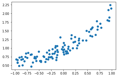
Polynomial Features
rng = np.random.RandomState(2)
x = rng.uniform(-1, 1, size=(100,))
X = x.reshape(-1, 1)
x_noisy = x + rng.normal(scale=0.1, size=x.shape)
coef = rng.normal(size=3)
y = coef[0] * x_noisy ** 2 + coef[1] * x_noisy + coef[2] + rng.normal(scale=0.1, size=x.shape)
plt.plot(x, y, 'o')
[<matplotlib.lines.Line2D at 0x7f4bdd31fda0>]
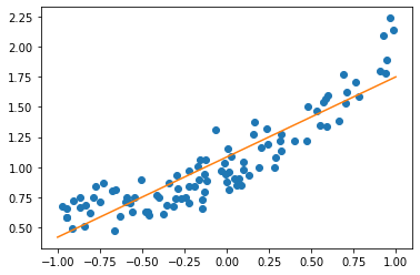
from sklearn.linear_model import LinearRegression
X_train, X_test, y_train, y_test = train_test_split(X, y, random_state=0)
lr = LinearRegression().fit(X_train, y_train)
line = np.linspace(-1, 1, 100).reshape(-1, 1)
plt.plot(x, y, 'o')
plt.plot(line, lr.predict(line))
lr.score(X_test, y_test)
0.7633239152617027
from sklearn.preprocessing import PolynomialFeatures
poly_lr = make_pipeline(PolynomialFeatures(include_bias=False), LinearRegression())

poly_lr.fit(X_train, y_train)

plt.plot(x, y, 'o')
plt.plot(line, lr.predict(line))
plt.plot(line, poly_lr.predict(line))
poly_lr.score(X_test, y_test)
0.8336786269754218

Feature Distributions
plt.boxplot(X_train_scaled)
plt.xticks(np.arange(1, X.shape[1] + 1), X.columns, rotation=30, ha="right");
plt.savefig("images/house_price_scaled_box.png")
fig, axes = plt.subplots(3, 6, figsize=(20, 10))
for i, ax in enumerate(axes.ravel()):
    if i > 16:
        ax.set_visible(False)
        continue
    ax.hist(X.iloc[:, i], bins=30)
    ax.set_title("{}: {}".format(i, X.columns[i]))
plt.savefig("images/house_price_hist.png")
def bc(x, l):
    if l == 0:
        return np.log(x)
    else:
        return (x ** l - 1) / l
line = np.arange(1e-10, 10, 100)
line
line = np.linspace(.01, 10, 100)
colors =  [plt.cm.viridis(i) for i in np.linspace(0, 1, 6)]
for l, c in zip([-1, -.5, 0, .5, 1, 2], colors):
    plt.plot(line, bc(line, l), label="lambda={}".format(l), color=c)
plt.ylim(-4, 6)
plt.gca().set_aspect("equal")
plt.legend(loc=(1, 0))
plt.xlim(0, 10)
from sklearn.preprocessing import MinMaxScaler
# this is very hacky and you probably shouldn't do this in real life.
X_train_mm = MinMaxScaler().fit_transform(X_train) + 1e-5
from sklearn.preprocessing import PowerTransformer
fig, axes = plt.subplots(3, 6, figsize=(20, 10))
pt = PowerTransformer()
X_bc = pt.fit_transform(X_train_mm)
print(pt.lambdas_)

for i, ax in enumerate(axes.ravel()):
    if i > 16:
        ax.set_visible(False)
        continue
    ax.hist(X_bc[:, i], bins=30)
    ax.set_title("{}: {} {:.2f}".format(i, X.columns[i], pt.lambdas_[i]))
plt.savefig("images/house_price_hist_boxcox.png")
X_bc_scaled = StandardScaler().fit_transform(X_bc)
fig, axes = plt.subplots(3, 6, figsize=(20, 10))
for i, ax in enumerate(axes.ravel()):
    if i > 16:
        ax.set_visible(False)
        continue
    ax.yaxis.set_major_formatter(million_formatter)
    ax.set_ylim(0, 4000000)
    ax.scatter(X_bc_scaled[:, i], y_train, s=.1, alpha=.1)
    ax.set_title("{}: {}".format(i, X.columns[i]))
    ax.set_ylabel("Progression")
plt.tight_layout()
plt.savefig("images/house_price_bc_scaled_scatter.png")
from sklearn.linear_model import RidgeCV
from sklearn.model_selection import cross_val_score

scores = cross_val_score(RidgeCV(), X_train, y_train, cv=10)
np.mean(scores), np.std(scores)
scores = cross_val_score(RidgeCV(), X_train_scaled, y_train, cv=10)
print(np.mean(scores), np.std(scores))
scores = cross_val_score(RidgeCV(), X_bc_scaled, y_train, cv=10)
np.mean(scores), np.std(scores)
ridge = RidgeCV().fit(X_train_scaled, y_train)
ridge_bc = RidgeCV().fit(X_bc_scaled, y_train)
plt.plot(ridge.coef_, 'o', label="scaled")
plt.plot(ridge_bc.coef_, 'o', label="box-cox")
plt.xlabel("coefficient index")
plt.ylabel("coefficient value")
plt.legend()
from sklearn.datasets import fetch_openml
data = fetch_openml("house_sales", as_frame=True)
data.frame.columns
data.frame.date
import dabl
dabl.plot(data.frame, target_col='price')