Working with Text data
Today, we’ll talk about working with text data.
FIXME CountVectorizer in Column transformer is weird, no list, just string. Example of combining text and non-text features. FIXME explain L2 normalization and intuition? FIXME BOW figure needs repainting FIXME hashing vectorizer slide missing score output FIXME a bit too long, remove european parliament example?
More kinds of data
So far:
Fixed number of features
Contiguous
Categorical
–
Next up:
No pre-defined features
Free text
Images
(Audio, video, graphs, …: not this class)
So far we talked about data where we have a fixed number of features, and where the features are either continuous or categorical. And that is most of the data out there and the simplest kind of data to work with.
The rest of the semester, we’re going to talk about different kinds of data that is opposite to what we already worked with.
We’ll look at data that has no predefined features. In particular, we’re going to look at free text and images. We’re also going to look at time series, which is a similar category of not having a clear way to express it as a standard supervised learning task. Another common example in this category is audio and video, we’re not going to do any audio or video in this lecture. But I think text and images are the common types of data.
Need to create fixed-length description
Typical Text Data
.center[
 ]
]
.center[
 ]
]
Here’s an example of some text dataset that I’m going to use later. This is like relatively typical text, its user input data from IMDb movie reviews.
Clearly, they don’t have the same length, there’s no clear way to express this is as like some floating point features which we would use for a standard machine learning approach. You can also see there are weird things about capitalization, some weird words in there like Godzilla that you might not see very often, there is some HTML markup, there’s punctuation and so on. This is sort of how text looks like in the wild very often. You could also do things on much longer texts, like whole books, or articles or so on.
People also work on text that’s much shorter. Tweets are still sort of their own domain. Working on tweets is quite hard because they are very short.
I’m going to talk about a particular kind of data that you see very often because it’s often used. But there are other kinds of data that is text data.
Other Types of text data
.center[
 ]
]
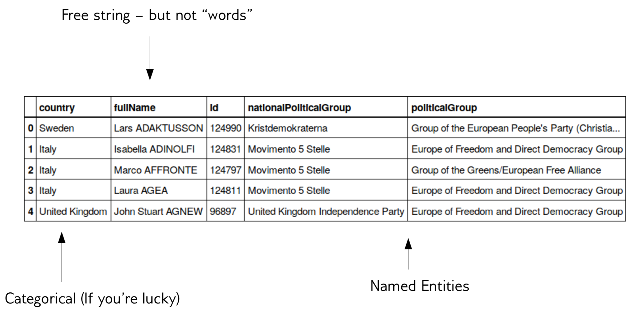
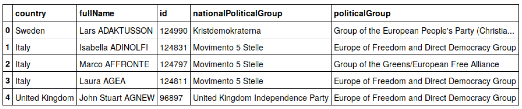
Here is a table of the text data consisting of people sitting in the European Parliament. Each person has a country, a name, an ID, a party, and a political affiliation. The variable country here, you might hope that it’s categorical but for the European Union, actually, the categories are well known. Though, if you have a user input a country, they will never input the same country in the same way. The UK could be the United Kingdom, or England, or Britain, or Great Britain, and all of these might correspond in this context to the same entity.
If you have users input this, they will also make typos. This variable is representing a category concept but you have to do some cleaning before you can actually convert it into a category. This is often a manual thing to do. There are things that can help you with this, like duplication or an entity recognition but we’re not going to talk about that.
The names are strings. They are definitely not categorical, and they’re also not words. So it’s not really clear if there’s like any information in the name and we’re going to look into this later today.
But you clearly don’t want to treat them the same way as words that you find in a dictionary.
We have the political groups and affiliations. Again, these are sort of free texts. They’re sort of similar to the variable country only now there’s many more of them, in a sense, they try to encode a categorical variable, which political group you’re from, but they also have more information, for example, you could also treat them as texts like if there’s freedom or democracy or Christianity or something in the party title that will probably say something. So you could either treat it as categorical or as text and both will give you information. And you have the same problem, that the same group can be referred with different names or different spellings.
So there’s this whole area of named entity recognition that actually tries to extract from any text the named entities and then tries to disambiguate. We’re actually going to talk about this, but it’s also some particular kind of text data that I want you to be aware of.
Bag of Words
.center[
 ]
]
The most common approach that people use for this is bag of words, which is a very simple approach.
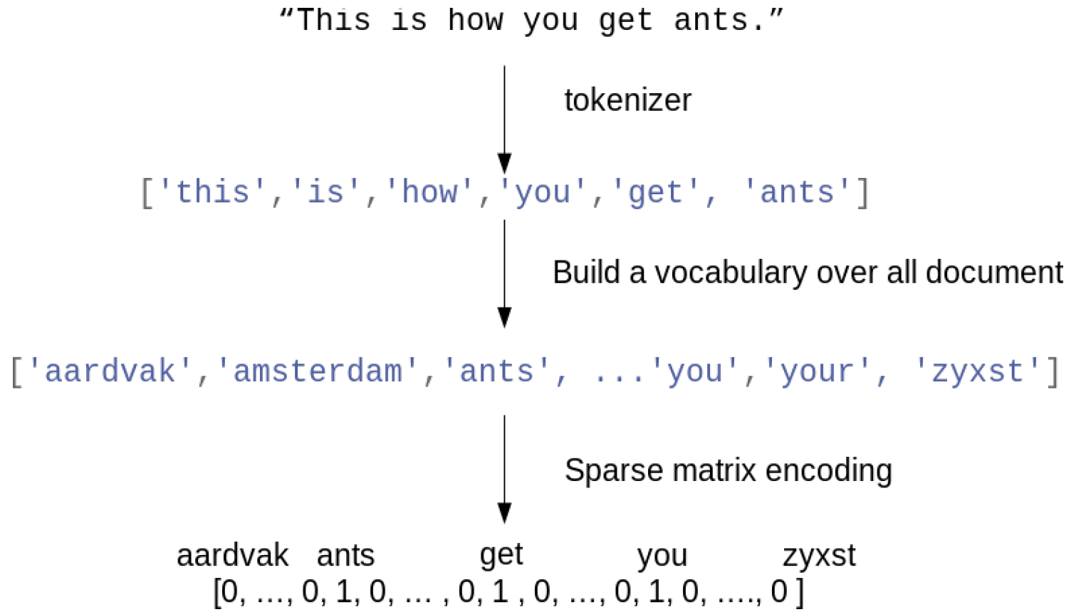
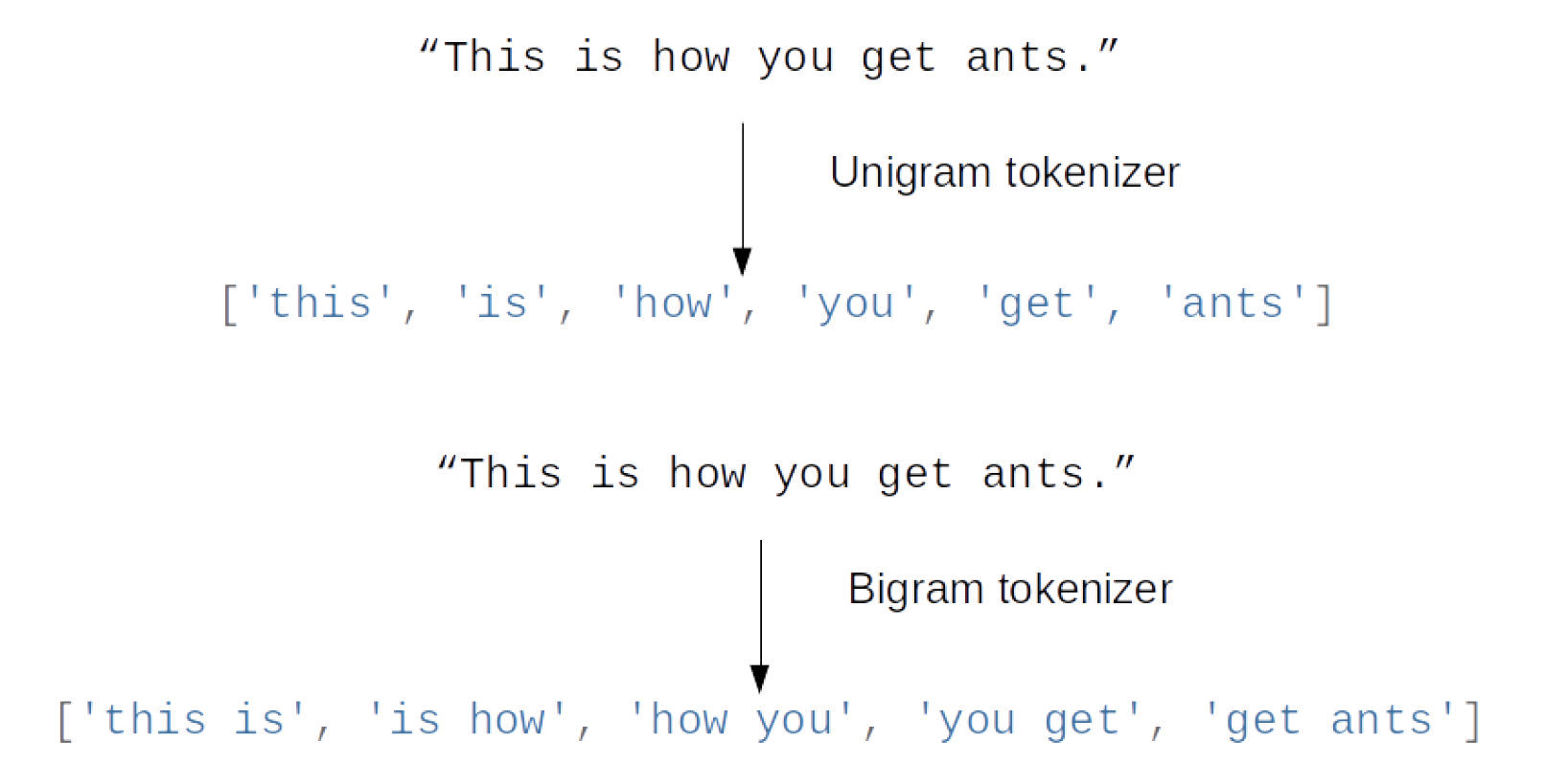
We start with a string which would be your whole document. The first step is to tokenize it, which is basically breaking it up the document into words. And then, you built a vocabulary over all documents over all words.
So you look over all the movie reviews, or all the emails or the text you have, and you collect all the tokens which are representing the words.
Finally, using the vocabulary, you create a group representation. The length of your feature vector will be the size of the vocabulary. For each word in the vocabulary, you count how often this word appears in the string that you want to encode.
Most of the words in the English language don’t appear in a sentence. So most of these entries will be 0. But the word ‘ants’ appears once, so increment the count for ‘ants’ by 1 and so on.
So I’ll have 6 non-zero entries and all the other entries will be 0. So this is what we call like a very sparse vector so most entries of this vector are 0.
When coding this, we’ll use a sparse matrix encoding. The idea of sparse matrix encoding is that you only store the non-zero entries.
So basically, we will only store the 1s, so storing the string as a bag of word will cost us a nearly 6 floating point numbers.
Toy Example
.smaller[
malory = ["Do you want ants?",
          "Because that’s how you get ants."]
from sklearn.feature_extraction.text import CountVectorizer
vect = CountVectorizer()
vect.fit(malory)
print(vect.get_feature_names())
['ants', 'because', 'do', 'get', 'how', 'that', 'want', 'you']
X = vect.transform(malory)
print(X.toarray())
array([[1, 0, 1, 0, 0, 0, 1, 1],
       [1, 1, 0, 1, 1, 1, 0, 1]])
]
Here, I have a corpus. Corpus is what people in NLP called datasets. My dataset is 2 strings, “Do you want ants?”, “Because that’s how you get ants.”
The bag of word representation is implemented in the count vectorizer in scikit-learn, which is a sklearn.feature_extraction.text
This is a transformer, it’s kind of similar to most transformers. The only difference is it takes in lists of strings as input, not numeric data. Usually, transformers take in a Numpy area as anything in scikit-learn.
But here, count vectorizer takes in a list of strings. I gave the list of string and I fit it on my documents and this builds the vocabulary. I can get back to vocabulary by looking at the feature names using get_feature_names()
The vocabulary is sorted alphabetically. Vocabulary has 8 entries from ‘ants’ to ‘you’. So if I use this count vectorizer to create like a word representation, then I’ll get an 8-dimensional feature space.
I can use this to transform the 2 documents that I have. X here, being the outcome of the transform will be a sparse matrix. So to print it, I call toarray() on it. So sparse matrices are in scipy, and you can easily convert to and from numpy arrays.
Usually, it’s a very bad idea to convert to sparse matrix into Numpy array, since usually, it will not fit into your memory. If you have like a vocabulary of size 100,000 and 100,000 documents, and you make it into Numpy array, then your memory will just fill up and your computer will crash since you won’t have enough memory to store all the zeros.
In this toy example, we can easily convert this to a Numpy array and you can see that this is the feature representation. In this case, we only have 1s and 0s.
Each word appears either once or zero times. So here, in the first string, the first feature is ‘ant’, so ‘ant’, ‘do’, ‘want’ and ‘you ’ appears once, ‘because’, ‘get’, ‘how’, and ‘that’ doesn’t appear. The second string is processed in the same way.
Q: What would you do if your document has more unique tokens or tokens that are not in the vocabulary?
Usually, you either ignore them, that’s the default thing to do. Your test set will have tokens that your training set will not have, and so you can’t really learn anything about that. One thing you could do is count how many words out of the vocabulary there are.
We going to talk a little bit later about how to restrict your vocabulary and you can basically add a new feature, that says, “There’s X amount of features that are not in the vocabulary.” Often, this can be useful for people cascading something or miss typing something or using names or something like that.
But usually, you assume that most of the words appear in your training data set.
Q: What if there are spelling errors?
You can treat them but by default, if you do that, they’re just different features. So they’re completely unrelated. So if there’s a new spelling error in your test dataset that never appeared in your training dataset, then the word will be completely ignored.
You can use spell correction, I’ll talk about that in a bit.
If you don’t do any spell correction, it will be a completely distinct feature. Spell correction is also not entirely trivial because there are many possible words.
Q: Does the count vectorizer trim the apostrophe in ‘that’s’ in the second string?
Yes, and as you can see, the question marks and the dots also don’t appear. And we’re going to talk about how exactly it works in a little bit.
Consider two documents in a dataset “malory”
“bag”
print(malory)
print(vect.inverse_transform(X)[0])
print(vect.inverse_transform(X)[1])
['Do you want ants?', 'Because that’s how you get ants.']
['ants' 'do' 'want' 'you']
['ants' 'because' 'get' 'how' 'that' 'you']
The reason why this is called a bag of words is since you’re completely ignoring the order of words. So you can do inverse transform to get back the string representation from the numerical representation but if you do that the numerical representation doesn’t contain the order of the words so you will only get back ‘ants’ ‘do’ ‘want’ ‘you’ and ‘ants’ ‘because’ ‘get’ ‘how’ ‘that’ ‘you’
Basically, you store all the words in a big bag and completely lose any context and any order of the words. That’s why it’s called a bag of words.
Text classification example:
IMDB Movie Reviews
We’re going to do a binary classification task on a dataset of IMDb movie reviews. You can look on GitHub, I have the notebook that runs through all of this if you want to run it yourself.
The idea here is that we want to do sentiment analysis basically classifying reviews into either being positive or negative. In IMDb, they give stars from 0 to 10. This is from a research paper where the author stated 1, 2 and 3 as negative while 7, 8, 9 and 10 are positive.
Data loading
from sklearn.datasets import load_files
reviews_train = load_files("../data/aclImdb/train/")

text_trainval, y_trainval = reviews_train.data, reviews_train.target
print("type of text_train: ", type(text_trainval))
print("length of text_train: ", len(text_trainval))
print("class balance: ", np.bincount(y_trainval))
type of text_trainval:

length of text_trainval: 25000
class balance: [12500 12500]
Text data is in either it’s in a CSV format or if they’re longer documents, people in NLP like to have a single text file for each data point.
There’s a tool in scikit-learn that allows you to load data, method load_files function, which basically iterates over all the folders in a given folder. Each folder is supposed to correspond to a class and then inside each folder, each text document corresponds to a data point, that’s a very common format that people use for text data.
We can load this, then we get the actual data and the targets.
Text_trainval is used as a training and validation set is just a list. The length is 25,000. So there are 25,000 documents, and this is a balanced dataset meaning there are 12,500 positive and negative samples.
Data loading
print("text_train[1]:")
print(text_trainval[1].decode())
.smaller[
text_train[1]:
'Words can't describe how bad this movie is. I can't explain it by
writing only. You have too see it for yourself to get at grip of how
horrible a movie really can be. Not that I recommend you to do that.
There are so many clichés, mistakes (and all other negative things
you can imagine) here that will just make you cry. To start with the
technical first, there are a LOT of mistakes regarding the airplane. I
won't list them here, but just mention the coloring of the plane. They
didn't even manage to show an airliner in the colors of a fictional
airline, but instead used a 747 painted in the original Boeing livery.
Very bad. The plot is stupid and has been done many times before, only
much, much better. There are so many ridiculous moments here that i
lost count of it really early. Also, I was on the bad guys' side all
the time in the movie, because the good guys were so stupid. "Executive
Decision" should without a doubt be you're choice over this one, even the
"Turbulence"-movies are better. In fact, every other movie in the world is
better than this one.'
]
We can also look at data points. I’m calling decode here to print the Unicode characters.
The word ‘cliché’ can be typed with or without the axon and they would be two different words. But also, you need to determine if it’s a Unicode character or not. In Python 3, by default, everything is a unique code.
Vectorization
text_train_val = [doc.replace(b"
", b" ")
                  for doc in text_train_val]
text_train, text_val, y_train, y_val = train_test_split(
    text_trainval, y_trainval, stratify=y_trainval, random_state=0)
vect = CountVectorizer()
X_train = vect.fit_transform(text_train)
X_val = vect.transform(text_val)
X_train
<
18750x66651 sparse matrix of type '
'
  with 2580448 stored elements in Compressed Sparse Row format>
I removed all the irrelevant HTML formatting. And then I split it into training and test set. Then I called the count vectorizer. Then I fitted the training set and transform the validation set.
Then it returns a 18750x66651 sparse matrix meaning there are 18,750 samples and 66,651 features.
So the vocabulary that we built is 66,651. There’s 2.5 million stored elements (non-zero entries).
This is a much, much smaller number than the product of these two numbers. So most of the entries are zero.
Remember, you need to know whether you are in Python 2 or 3 and then you need to know the type of text.
There are two different things that you need to keep in mind. So the text can be a byte string or Unicode string. But if it’s a byte string, it also has an encoding attached with it. You need to know the encoding to go from the byte string to the string.
Vocabulary
feature_names = vect.get_feature_names()
print(feature_names[:10])
.smaller[
['00', '000', '0000000000001', '00001', '00015', '000s', '001', '003830', '006', '007']
]
print(feature_names[20000:20020])
.smaller[
['eschews', 'escort', 'escorted', 'escorting', 'escorts', 'escpecially', 'escreve',
 'escrow', 'esculator', 'ese', 'eser', 'esha', 'eshaan', 'eshley', 'esk', 'eskimo',
 'eskimos', 'esmerelda', 'esmond', 'esophagus']
]
print(feature_names[::2000])
.smaller[
['00', 'ahoy', 'aspects', 'belting', 'bridegroom', 'cements', 'commas', 'crowds',
 'detlef', 'druids', 'eschews', 'finishing', 'gathering',  'gunrunner', 'homesickness',
 'inhumanities', 'kabbalism', 'leech', 'makes', 'miki', 'nas', 'organ', 'pesci',
 'principally', 'rebours', 'robotnik', 'sculptural', 'skinkons', 'stardom', 'syncer',
 'tools', 'unflagging', 'waaaay', 'yanks']
]
This is the first thing I do, it’s helpful to see if something sensible happened. And you get an idea of the data. I’m going to plot the first 10 data points, and I’m going to plot some 20 in the middle and I’m going to plot every 2000th data point.
The first couple of ones seem to be pretty boring. But then it seems to do something relatively reasonable.
Now that we have the sparse matrix representation, we can just do classification as usual.
Classification
from sklearn.linear_model import LogisticRegressionCV
lr = LogisticRegressionCV().fit(X_train, y_train)
lr.C_
array([ 0.046])
lr.score(X_val, y_val)
0.882
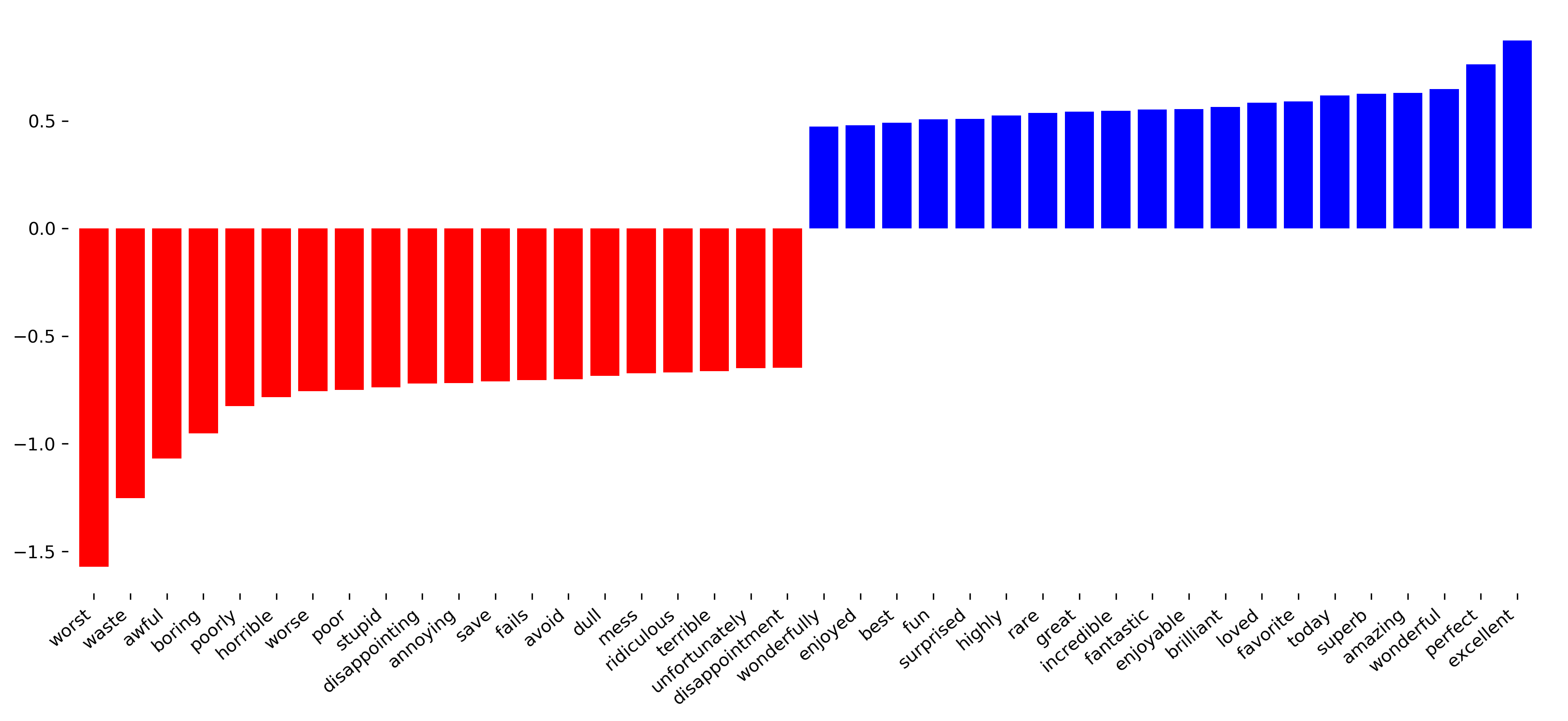
All the models in scikit-learn work directly on the sparse matrix representation. Here, I do logistic regression CV so it adjusts CR automatically for me. The validation set score I get is 88% accuracy, which is pretty good.
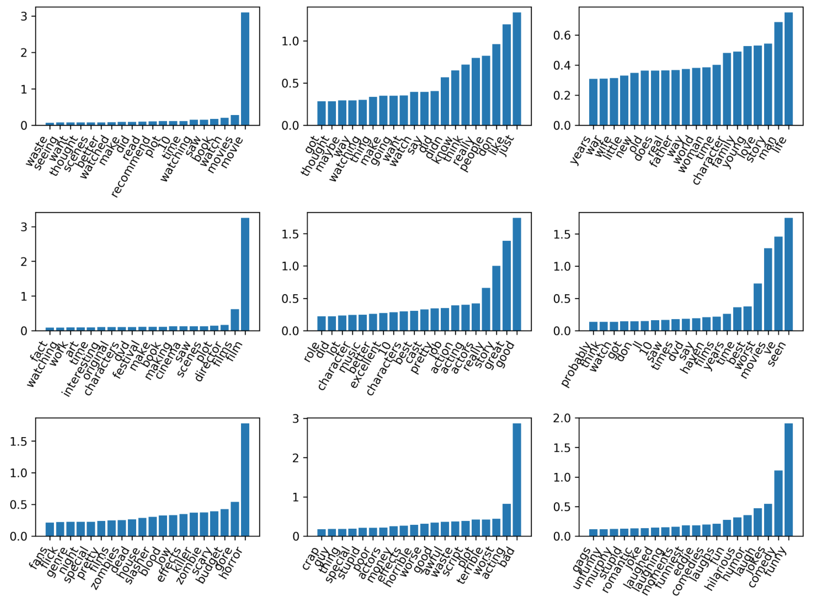
Here, accuracy is meaningful because we know it’s a balanced dataset. The next thing I always like to do is look at the coefficients.
.center[
 ]
]
So here I’m looking at the 20 most negative and 20 most positive coefficients of this logistic regression. It’s pretty easy to do because it’s a binary task. If you have multiclass tasks, you’ll have way more coefficients and it’s harder to visualize.
This seems to be like a pretty reasonable model to pick up on the bad words and the good words. This is the baseline approach.
Soo many options!
How to tokenize?
How to normalize words?
What to include in vocabulary?
In tokenization, there are many different options to change what’s happening here.
In particular, there’s the tokenization, which is how do you break it up into tokens. Then normalization, which is how do you make tokens look sort of reasonable. And then what to include in vocabulary.
Tokenization
Scikit-learn (very simplistic):
re.findall(r"\b\w\w+\b")Includes numbers
discards single-letter words
-or'break up words
Scikit-learn is not an LLP library. Some very good Python LLP libraries are NLTK and spacy. They have a lot more things for doing text analysis. Scikit-learn only has quite simple things.
In tokenization, what the count vectorizer does the regular expression, “\b\w\w+\b”. That means it finds anything of length 2 or longer that has word boundaries, which are any punctuation or white spaces, and matches w.
As we saw, this includes any numbers. Numbers can be at the beginning of the word, the middle of the word or it can be just all numbers.
You don’t include single letter work or single letter numbers. So ‘I’ is always discarded. There’s an interesting thing where you can get the gender of a person, depending on how much often they use ‘I’.
It doesn’t include any punctuation because we only use the w, which is digits.
This is pretty simple and pretty restrictive.
Changing the token pattern regex
vect = CountVectorizer(token_pattern=r"\b\w+\b")
vect.fit(malory)
print(vect.get_feature_names())
['ants', 'because', 'do', 'get', 'how', 's', 'that', 'want', 'you']
–
vect = CountVectorizer(token_pattern=r"\b\w[\w’]+\b")

vect.fit(malory)
print(vect.get_feature_names())
['ants', 'because', 'do', 'get', 'how', 'that’s', 'want', 'you']
If we just want to use a different regular expression, we can do something simple, like changing the regular expression. So here, for example, I removed one of the Ws and so now I match everything that’s a single letter or more. So now I only the ‘s’ in ‘that’s’, without the apostrophe, making it a single token.
I can also allow things to have an apostrophe in the middle of the word, and get ‘that’s’ as a single token. This might look nicer but actually, in reality, it usually doesn’t matter that much.
But you can play around with this and see if the tokens you get with standard tokenization are good for your application.
Again, spacy and NLTK have much more sophisticated things. The X in vectorization slide represents the sparse matrix representation of the data and Y represents if it’s a positive or a negative review.
Was not actually an apostroph but some unicode pattern because I copy & pasted the quote.
#Normalization
.smaller[
Correct spelling?
Stemming: reduce to word stem
Lemmatization: smartly reduce to word stem ] – .smaller[ “Our meeting today was worse than yesterday,
I’m scared of meeting the clients tomorrow.”
Stemming:
['our', 'meet', 'today', 'wa', 'wors', 'than', 'yesterday', ',', 'i', "'m", 'scare', 'of', 'meet', 'the', 'client', 'tomorrow', '.']
Lemmatization:
['our', 'meeting', 'today', 'be', 'bad', 'than', 'yesterday', ',', 'i', 'be', 'scar', 'of', 'meet', 'the', 'client', 'tomorrow', '.']
]
.smaller[
scikit-learn:
Lower-case it
Configurable, use nltk or spacy ]
Normalization is basically how do you want to bring your token in a standardized form. For example, you could get rid of plurals or you could correct spelling. There are three main methods.
Correct spelling, which only very few people use in practice.
Stemming reduces words to their word stem. The idea is to get rid of plural ‘s’ and ‘ing’ at the end of the verbs and so on so that you don’t have the conjugations. Stemming removes some letters at the end of the word depending on a fixed rule set.
Lemmatization also uses reduces the word stem but in a smart way. It tries to parse the sentence and then uses a dictionary of all English words with all its verb forms and conjugations and tries to map it to a standardized form.
The reason why I picked this example is ‘meeting’ appears twice in here, once as a noun and once as a verb. Using stemming: ‘was’ becomes ‘wa’ ‘worse’ becomes ‘wors’ and so on ‘I’m’ is just split up in two without the apostrophe. ‘scared’ becomes ‘scare’ ‘meeting’ becomes ‘meet’
Lemmatization parsed the sentence and figured out that the first ‘meeting’ is a noun and keeps it as it is but the second ‘meeting’ which is a verb is simplified to ‘meet’. You can also see that the ‘was’ was normalized to ‘be’ and the ‘worse’ was normalized to ‘bad’ and the ’m was normalized to ‘be’ as well.
The question with any kind of normalization you do is will this be helpful for your application.
Q: is stemming only applicable to English literature?
These are both language dependent. This model exists for many languages. Today, I’m only talking about languages that work similar to English.
Scikit-learn only lowercases it. You can plug in other normalization from NLTK or spacy into the count vectorizer if you want, but the default is it lower cases the tokens.
Restricting the Vocabulary
The other main thing that you can play with is restricting the vocabulary. So far, I said, we’re just going to use all the tokens that we see.
Stop Words
vect = CountVectorizer(stop_words='english')
vect.fit(malory)
print(vect.get_feature_names())
['ants', 'want']
from sklearn.feature_extraction.text import ENGLISH_STOP_WORDS
print(list(ENGLISH_STOP_WORDS))
.tiny-code[
['former', 'above', 'inc', 'off', 'on', 'those', 'not', 'fifteen', 'sometimes', 'too', 'is', 'move', 'much', 'own', 'until', 'wherein',
'which', 'over', 'thru', 'whoever', 'this', 'indeed', 'same', 'three', 'whatever', 'us', 'somewhere', 'after', 'eleven', 'most', 'de', 'full',
'into', 'being', 'yourselves', 'neither', 'he', 'onto', 'seems', 'who', 'between', 'few', 'couldnt', 'i', 'found', 'nobody', 'hereafter',
'therein', 'together', 'con', 'ours', 'an', 'anyone', 'became', 'mine', 'myself', 'before', 'call', 'already', 'nothing', 'top', 'further',
'thereby', 'why', 'here', 'next', 'these', 'ever', 'whereby', 'cannot', 'anyhow', 'thereupon', 'somehow', 'all', 'out', 'ltd', 'latterly',
'although', 'beforehand', 'hundred', 'else', 'per', 'if', 'afterwards', 'any', 'since', 'nor', 'thereafter', 'it', 'around', 'them',
'alone', 'up', 'sometime', 'very', 'give', 'elsewhere', 'always', 'cant', 'due', 'forty', 'still', 'either', 'was', 'beyond', 'fill',
'hereupon', 'no', 'might', 'by', 'everyone', 'five', 'often', 'several', 'and', 'something', 'formerly', 'she', 'him', 'become', 'get',
'could', 'ten', 'below', 'had', 'how', 'back', 'nevertheless', 'namely', 'herself', 'none', 'be', 'himself', 'becomes', 'hereby',
'never', 'along', 'while', 'side', 'amoungst', 'toward', 'made', 'their', 'part', 'everything', 'his', 'becoming', 'a', 'now', 'am',
'perhaps', 'moreover', 'seeming', 'themselves', 'name', 'etc', 'more', 'another', 'whither', 'see', 'herein', 'whom', 'among', 'un', 'via',
'every', 'cry', 'me', 'should', 'its', 'again', 'co', 'itself', 'two', 'yourself', 'seemed', 'under', 'then', 'meanwhile', 'anywhere',
'beside', 'seem', 'please', 'behind', 'sixty', 'were', 'in', 'upon', 'than', 'twelve', 'when', 'third', 'to', 'though', 'hence',
'done', 'other', 'where', 'someone', 'of', 'whose', 'during', 'many', 'as', 'except', 'besides', 'for', 'within', 'mostly', 'but',
'nowhere', 'we', 'our', 'through', 'both', 'bill', 'yours', 'less', 'well', 'have', 'therefore', 'one', 'last', 'throughout', 'can',
'mill', 'against', 'anyway', 'at', 'system', 'noone', 'that', 'would', 'only', 'rather', 'wherever', 'least', 'are', 'empty', 'almost',
'latter', 'front', 'my', 'amount', 'put', 'what', 'whereas', 'across', 'whereupon', 'otherwise', 'thin', 'others', 'go', 'thus',
'enough', 'her', 'fire', 'may', 'once', 'show', 'because', 'ourselves', 'some', 'such', 'yet', 'eight', 'sincere', 'from', 'been', 'twenty',
'whether', 'without', 'you', 'do', 'everywhere', 'six', 'however', 'first', 'find', 'hers', 'towards', 'will', 'also', 'even', 'or',
're', 'describe', 'serious', 'so', 'anything', 'must', 'ie', 'the', 'whenever', 'thick', 'bottom', 'they', 'keep', 'your', 'has', 'about',
'each', 'four', 'eg', 'interest', 'hasnt', 'detail', 'amongst', 'take', 'thence', 'down', 'fifty', 'whence', 'whereafter', 'nine', 'with',
'whole', 'there']
]
One way to restrict the vocabulary often is to remove stop words. Stop words, are words that are not so important to the content and so you discard them.
If I do this for my example, the only thing that remains are ‘ants’ and ‘want’ because ‘this’, ‘I’ and ‘how’ are all stop words.
Scikit-learn has some stop words built in. So if you do stop word equal to English, it will use the built-in the stop word list. It’s a little bit strange and we’re working on improving it. So for example, there’s ‘system’ in the stop word list and ‘bill’ is in the stop word list.
For unsupervised problems, using stop words might be helpful. For supervised problems, I rarely found it helpful with the tools that we talked about.
So problem is, these are nearly 200 words but we have 66,000 features, removing 200 features doesn’t really make a difference. And because these words appear very often, the model won’t be able to figure out are they important or not.
If you use an unsupervised model, in the unsupervised model since they appear so often, these might just dominate whatever clustering you do and so removing them might be a good idea.
not a very good stop-word list? Why is system in it? bill?
For supervised learning often little effect on large corpuses (on small corpuses and for unsupervised learning it can help)
Infrequent Words
Remove words that appear in less than 2 documents:
.smaller[
vect = CountVectorizer(min_df=2)
vect.fit(malory)
print(vect.get_feature_names())
['ants', 'you']
]
Restrict vocabulary size to max_features most frequent words:
.smaller[
vect = CountVectorizer(max_features=4)
vect.fit(malory)
print(vect.get_feature_names())
['ants', 'because', 'do', 'you']
]
Another thing that is often helpful is removing infrequent words. There’s a parameter called min_df that basically removes words that appear less than twice.
It’ll only keep words that appeared twice or more, and so only ‘ants’ and ‘you’ remain in the toy dataset example.
This is often useful because it can remove a lot of features. And if a word appears only once in your data, it’s unlikely that your algorithm will be able to learn. If you have hundreds of thousands of thousands of features, and one feature appears once in your dataset, then it’s probably not going to be helpful.
You can also go the other way around and set max_features. Max_features sets the number of features that you want to keep, in this case, four most common features.
It’s kind of interesting, this goes a little bit in the opposite direction of what the stop words do. The stop words remove the most common ones that are meaningless and here, we removed the most infrequent ones because they’re probably not helpful. These are often misspellings, or names or something like that.
.smaller[
vect = CountVectorizer(min_df=2)
X_train_df2 = vect.fit_transform(text_train)

vect = CountVectorizer(min_df=4)
X_train_df4 = vect.fit_transform(text_train)
X_val_df4 = vect.transform(text_val)

print(X_train.shape)
print(X_train_df2.shape)
print(X_train_df4.shape)
(18750, 66651)
(18750, 39825)
(18750, 26928)
lr = LogisticRegressionCV().fit(X_train_df4, y_train)
lr.C_
array([ 0.046])
lr.score(X_val_df4, y_val)
0.881
]
Here I used the count vectorizer with min_df=2 and min_df=4. That means either use tokens that appear in 2 documents in a training set, or at least 4 documents in a training set.
Min_df=2 gives me 39825 while min_df=4 gives me 26928. I’ve drastically reduced the feature space when using min_df=2 and if I set min_df=4, I cut down feature space even more.
Min_df means minimum document frequency, meaning the number of documents the words appear in. It’s not the number of times the word appears. So if a word appears in 100 times in a single document, it’s still going to be thrown out by this.
Here, I used X_train_df=4, which is much, much smaller, it’s less than half the size. And the result I get is identical, basically, in terms of accuracy.
These are the main configuration you just used a single bag of words.
That said, they’re throwing away a lot of the context and information. One way to improve upon this is what’s called N-grams.
Removed nearly 1/3 of features!
As good as before
Tf-idf rescaling
\(n_d\) = total number of documents
\(df(d,t)\) = number of documents containing term \(t\)
–
In sklearn: by default also L2 normalisation!
Next thing we can do is actually try to rescale our words with something called Tf-idf which stands for Term Frequency Inverse Document Frequency.
This is sort of an alternative to using soft stop words in a sentence. The idea here is to down-weight things that are very common.
It’s the logarithm of 1 over the number of documents containing the term.
So if something happens to appear in most of the documents, the inverse document frequency will give it a very low weight. This is something that’s very commonly used in information retrieval.
Information retrieval basically means you’re trying to find relevant documents. If you can think of how a search engine works, if you want to match a bag of words representation of two different query strings, you might not care so much about matching the ‘a’ and ‘the’, but you care a lot about matching the parts that are rare and that are very specific to a particular search term. That is the motivation for this.
But people find it also sometimes helps in a machine learning context.
You can’t really know in advance whether this helps for the particular dataset or not, but basically you should keep in mind, this emphasizes rare words and does a soft removal of very common words. This also means the sort of stop words here are corpus specific so here it will learn to down-weight ‘movie’ and ‘film’ because they’re very common.
The implementation of this in scikit-learn is a little bit non-standard but I don’t think it makes a big difference.
You should also keep in mind is that if you use the implementation of TF-IDF in scikit-learn by default, it will also do L2 normalization. L2 normalization means you divide each row by its length. That means you normalize the weight the length of the document. You only want to count how often the word appears relative to how long the document is. Basically, if you make a document that basically repeats each word twice, it should still have the same representation. By default, that’s turned on for TF-IDF. But it’s not turned on for the bag of words.
Emphasizes “rare” words - “soft stop word removal”
Slightly non-standard smoothing (many +1s)
TfidfVectorizer, TfidfTransformer
.smaller[
from sklearn.feature_extraction.text import TfidfVectorizer, TfidfTransformer
malory_tfidf = TfidfVectorizer().fit_transform(malory)
malory_tfidf.toarray()
array([[ 0.41 ,  0.   ,  0.576,  0.   ,  0.   ,  0.   ,  0.576,  0.41 ],
       [ 0.318,  0.447,  0.   ,  0.447,  0.447,  0.447,  0.   ,  0.318]])
malory_tfidf = make_pipeline(CountVectorizer(),
                             TfidfTransformer()).fit_transform(malory)
malory_tfidf.toarray()
array([[ 0.41 ,  0.   ,  0.576,  0.   ,  0.   ,  0.   ,  0.576,  0.41 ],
       [ 0.318,  0.447,  0.   ,  0.447,  0.447,  0.447,  0.   ,  0.318]])
]
In scikit-learn, there are two ways to do this. You can either use the TF-IDF vectorizer which you can use directly on the text and it will build the vocabulary and then do the rescaling. Or you can use to count vectorizer, TFIDFTransformer, which will work on the sparse matrix created by the count vectorizer and then just transform it using rescaling.
This is an alternative to using stop words or putting more emphasis on rare words.
Q: Explain the part about the L2 norm.
For the L1 norm, it might be easier to visualize. Dividing by L1 norm would mean just dividing by word count and so that would mean that basically, if you have a very long review, and it says bad 3 times, but it says good 20 times, then you only care about the relative frequency. And if it’s a very short review that says good, 0 times, and bad also 3 times, then it’s probably a bad review. So you want to really scale these so that the relative frequency of the word only matters and not the total length document. That’s sort of what the normalization does.
And so the common thing to do is L2 normalization, which divides by Euclidean norm.
N-grams: Beyond single words
Bag of words completely removes word order.
“didn’t love” and “love” are very different!
–
.center[
 ]
]
Because there’s a big difference between ‘didn’t love’ and ‘love’ and the default settings in the count vectorizer cannot distinguish between the two because somewhere along the document, it could appear ‘don’t’ and you don’t know if it’s in front of ‘love’, or if it’s ‘love, don’t hate’ or ‘don’t love hate’, since they basically have the same representation.
The idea behind N-grams is you look at pairs of words that appear next to each other. Unigrams looks at single words, bigrams look at pairs of two words next to each other, and trigrams looks at three words next to each other, and so on.
Here instead of splitting it up into single tokens, we can split it up into pairs of tokens allowing me to have a little bit of context around each of the words.
N-grams: tuples of consecutive words
Bigrams toy example
.tiny-code[
cv = CountVectorizer(ngram_range=(1, 1)).fit(malory)
print("Vocabulary size: ", len(cv.vocabulary_))
print("Vocabulary:\n", cv.get_feature_names())
Vocabulary size: 8
Vocabulary:
['ants', 'because', 'do', 'get', 'how', 'that', 'want', 'you']
cv = CountVectorizer(ngram_range=(2, 2)).fit(malory)
print("Vocabulary size: ", len(cv.vocabulary_))
print("Vocabulary:\n", cv.get_feature_names())
Vocabulary size: 8
Vocabulary:
['because that', 'do you', 'get ants', 'how you', 'that how', 'want ants', 'you get', 'you want']
cv = CountVectorizer(ngram_range=(1, 2)).fit(malory)
print("Vocabulary size: ", len(cv.vocabulary_))
print("Vocabulary:\n", cv.get_feature_names())
Vocabulary size: 16
Vocabulary:
['ants', 'because', 'because that', 'do', 'do you', 'get', 'get ants', 'how', 'how you', 'that', 'that how', 'want', 'want ants',
'you', 'you get', 'you want']
]
When implementing in scikit-learn, you have to specify the N-gram range, which has the minimum number of tokens and the maximum number of tokens you want to look at.
Usually, you want to look at Unigram + Bigrams + Trigrams, don’t look at only Bigrams. If I only look at Unigrams, I get a vocabulary of size 8. If I look only at Bigrams, I get a vocabulary of size 8 as well, that’s because this was a toy example and in the real world there will be much more Bigrams than Unigrams.
If you look at the result from combining Unigrams and Bigrams together, we get 16, which is a combination of both the result.
Now I have a feature representation of size 16, and so I extended my feature space so that I can take the context into account.
Unigrams and Bigrams together are the most common combinations. Using higher order N-grams is rare.
Typically: higher n-grams lead to blow up of feature space!
N-grams on IMDB data
Vocabulary Sizes
1-gram (min_df=4): 26928
2-gram (min_df=4): 128426
1-gram & 2-gram (min_df=4): 155354
1-3gram (min_df=4): 254274
1-4gram (min_df=4): 289443
cv = CountVectorizer(ngram_range=(1, 4)).fit(text_train)
print("Vocabulary size 1-4gram: ", len(cv.vocabulary_))
Vocabulary size 1-4gram (min_df=1): 7815528
More than 20x more 4-grams!
This is using no stop words.
Now because many bigrams and many trigrams are very infrequent. So if I use the example of min_df=4 in Unigrams I get 26928 features while in Bigrams I get 128426 features. So it grew by nearly the order of magnitude. So I have a much, much bigger feature space now. If I put it together, it’s even bigger.
The higher I go, the bigger it gets. Though, you can see that it actually grows relatively slowly here. So if I look into 1-3grams programs, and 1-4grams, I only get 300,000 features. But this is mostly because I did the min_df=4. There are very few sequences of 4 words that appear often together. If I don’t use the min_df=4 and I look at all things I get nearly 8 million features. This is like 20 times more four grams than what we had before.
So particularly if you use higher N-grams using this pruning of document frequency might be quite helpful. You can see that probably they have about the same amount of information, but you’ll have 20 times fewer features, which will definitely impact runtime and possibly impact generalization.
#Stop-word impact on bi-grams
cv = CountVectorizer(ngram_range=(1, 2), min_df=4)
cv.fit(text_train)
print("(1, 2), min_df=4: ", len(cv.vocabulary_))
cv = CountVectorizer(ngram_range=(1, 2), min_df=4,
                     stop_words="english")
cv.fit(text_train)
print("(1, 2), stopwords, min_df=4: ", len(cv.vocabulary_))
(1, 2), min_df=4: 155354
(1, 2), stopwords, min_df=4: 81085
This is with stop words. What we’re doing is we do stop words first and then N-grams. What I find interesting is that here using unigrams and bigrams we got 155354, but if we remove the stop words it gets halved to 81085. This is pretty extreme.
The stop word list is only 200 words. So if we remove these 200 words and if you look at the bigrams we half the number of bigrams. This is because the most common combinations are actually we with stop words. So ‘the movie’ and ‘the film’ are probably the most common Bigrams in this.
So if we remove this then whatever word that came before ‘the’ is now makes after bigram. And so now, the combinations appear much less frequently.
Stop-word impact on 4-grams
cv4 = CountVectorizer(ngram_range=(4, 4), min_df=4)
cv4.fit(text_train)
cv4sw = CountVectorizer(ngram_range=(4, 4), min_df=4,
                       stop_words="english")
cv4sw.fit(text_train)
print(len(cv4.get_feature_names()))
print(len(cv4sw.get_feature_names()))```
31585 369
4grams are even rarer and so there are 31585 4grams that
appear at least 4 times but if I remove the stop words I get
only 369 4grams that appeared at least 4 times.
+++
[‘worst movie ve seen’ ‘40 year old virgin’ ‘ve seen long time’ ‘worst movies ve seen’ ‘don waste time money’ ‘mystery science theater 3000’ ‘worst film ve seen’ ‘lose friends alienate people’ ‘best movies ve seen’ ‘don waste time watching’ ‘jean claude van damme’ ‘really wanted like movie’ ‘best movie ve seen’ ‘rock roll high school’ ‘don think ve seen’ ‘let face music dance’ ‘don say didn warn’ ‘worst films ve seen’ ‘fred astaire ginger rogers’ ‘ha ha ha ha’ ‘la maman et la’ ‘maman et la putain’ ‘left cutting room floor’ ‘ve seen ve seen’ ‘just doesn make sense’ ‘robert blake scott wilson’ ‘late 70 early 80’ ‘crouching tiger hidden dragon’ ‘low budget sci fi’ ‘movie ve seen long’ ‘toronto international film festival’ ‘night evelyn came grave’ ‘good guys bad guys’ ‘low budget horror movies’ ‘waste time watching movie’ ‘vote seven title brazil’ ‘bad bad bad bad’ ‘morning sunday night monday’ ‘14 year old girl’ ‘film based true story’ ‘don make em like’ ‘silent night deadly night’ ‘rating saturday night friday’ ‘right place right time’ ‘friday night friday morning’ ‘night friday night friday’ ‘friday morning sunday night’ ‘don waste time movie’ ‘saturday night friday night’ ‘really wanted like film’]
This is the most common 4grams after removing stop words.
Whenever you have the ability to look into something
interesting in our data, do it.
+++
.center[

]
.center[

]
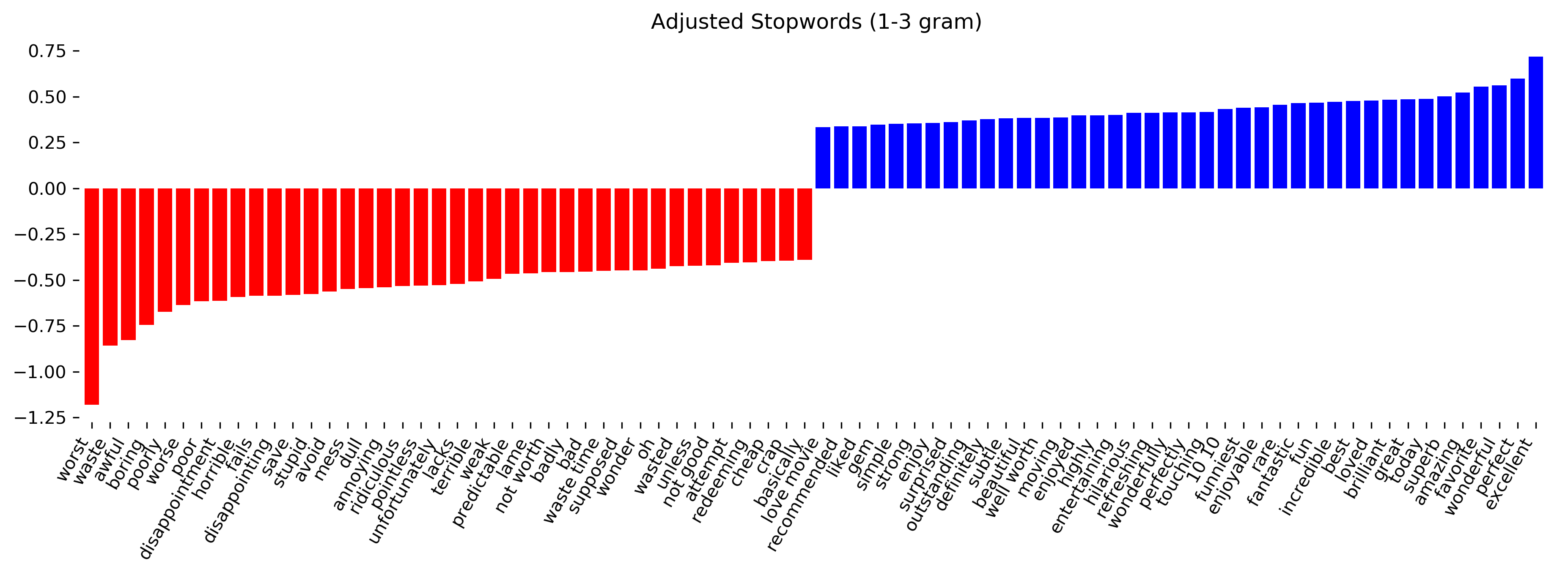
Here are some models using Unigrams, Bigrams, and Trigrams,
with and without stop words. You can see that most of the
most common features are actually Unigrams.
It's interesting because previously ‘worth’ didn't show up
but since we have bigrams, we can distinguish between ‘not
worth’ and ‘well worth’.
You can also see that most of these actually were Bigrams
that included stop word.
It gets slightly worse because all of these Bigrams actually
have stop words in them.
Stopwords removed fares slightly worse
+++
.tiny-code[
```python
my_stopwords = set(ENGLISH_STOP_WORDS)
my_stopwords.remove("well")
my_stopwords.remove("not")
my_stopwords.add("ve")
vect3msw = CountVectorizer(ngram_range=(1, 3), min_df=4, stop_words=my_stopwords)
X_train3msw = vect3msw.fit_transform(text_train)
lr3msw = LogisticRegressionCV().fit(X_train3msw, y_train)
X_val3msw = vect3msw.transform(text_val)
lr3msw.score(X_val3msw, y_val)
0.883
]
.center[
 ]
]
Basically, removing stop words is fine but you should keep in the ‘not’ and the ‘well’ so that the important things can still be expressed.
Character n-grams
The next thing I want to talk about is character n-grams. Character n-grams are a different way to extract features from text data. It’s not that useful for general text classification but it’s useful for some more specific applications.
The idea is that, instead of looking at tokens, which are words, we look at windows of characters.
#Principle
.center[
 ]
]
#Principle
.center[
 ]
]
#Principle
.center[
 ]
]
#Principle
.center[
 ]
]
#Principle
.center[
 ]
]
Here, I want to look at character trigrams, look at windows of length 3.
My first one would be “Do_” and then “o_y” and then “_you” and so…
Then you build the vocabulary over these trigrams.
#Applications
Be robust to misspelling / obfuscation
Language detection
Learn from Names / made-up words
This can be helpful to be more robust towards misspelling or obfuscation. So people might replace a single particular letter in a word with like internet speak. And so if you use character n-grams, you can still match if someone used the same characters for the rest of the word.
You can also use it for language detection. Language detection, I think by now relatively soft task. But basically, it’s very easy to detect the language, if you have a text, you can use character n-grams. You can’t really use a bag of words because the words in different languages are sort of distinct, and you don’t actually need to build vocabularies for all the languages. If you just look at the n-grams, that’s enough to know whether something is English or French or something.
Also, it helps to learn from names or any made-up words.
One thing that is interesting in a social context is to look at ethnicity from names. And you can actually get someone’s ethnicity from their last name, and in some cases, also from their first name.
Toy example
“Naive”
.tiny-code[
cv = CountVectorizer(ngram_range=(2, 3), analyzer="char").fit(malory)
print("Vocabulary size: ", len(cv.vocabulary_))
print("Vocabulary:\n", cv.get_feature_names())
Vocabulary size: 73
Vocabulary:
[' a', ' an', ' g', ' ge', ' h', ' ho', ' t', ' th', ' w', ' wa', ' y', ' yo', 'an', 'ant', 'at', 'at’', 'au', 'aus', 'be', 'bec', 'ca',
'cau', 'do', 'do ', 'e ', 'e t', 'ec', 'eca', 'et', 'et ', 'ge', 'get', 'ha', 'hat', 'ho', 'how', 'nt', 'nt ', 'nts', 'o ', 'o y', 'ou',
'ou ', 'ow', 'ow ', 's ', 's h', 's.', 's?', 'se', 'se ', 't ', 't a', 'th', 'tha', 'ts', 'ts.', 'ts?', 't’', 't’s', 'u ', 'u g', 'u w',
'us', 'use', 'w ', 'w y', 'wa', 'wan', 'yo', 'you', '’s', '’s ']
]
Respect word boundaries
.tiny-code[
cv = CountVectorizer(ngram_range=(2, 3), analyzer="char_wb").fit(malory)
print("Vocabulary size:", len(cv.vocabulary_))
print("Vocabulary:\n", cv.get_feature_names())
Vocabulary size: 74
Vocabulary:
[' a', ' an', ' b', ' be', ' d', ' do', ' g', ' ge', ' h', ' ho', ' t', ' th', ' w', ' wa', ' y', ' yo', '. ', '? ', 'an', 'ant', 'at', '
at’', 'au', 'aus', 'be', 'bec', 'ca', 'cau', 'do', 'do ', 'e ', 'ec', 'eca', 'et', 'et ', 'ge', 'get', 'ha', 'hat', 'ho', 'how', 'nt', 'nt ',
'nts', 'o ', 'ou', 'ou ', 'ow', 'ow ', 's ', 's.', 's. ', 's?', 's? ', 'se', 'se ', 't ', 'th', 'tha', 'ts', 'ts.', 'ts?', 't’', 't’s',
'u ', 'us', 'use', 'w ', 'wa', 'wan', 'yo', 'you', '’s', '’s ']
]
To do this with scikit-learn, you can use the count vectorizer with the analyzer equal char. So instead of word tokenization, it does character tokenization.
Usually, we look at characters that are longer, so single characters don’t really tell us much. Here, I look at n-grams of size 2 and 3. You can also go up to, like 5 or 7, obviously, the feature space tends to explode if you go higher.
After applying, I get a vocabulary of size 73, which is pretty big for such a short text.
And there’s also a featurette that can respect word boundaries called char_wb.
So here, you get the end of one word and the beginning of the next word, you might want to exclude that if you’re only interested on the actual words. So the char_wb makes sure that there’s no white space inside the character n-gram.
IMDB Data
.smaller[
char_vect = CountVectorizer(ngram_range=(2, 5), min_df=4, analyzer="char_wb")
X_train_char = char_vect.fit_transform(text_train)
len(char_vect.vocabulary_)
164632
lr_char = LogisticRegressionCV().fit(X_train_char, y_train)
X_val_char = char_vect.transform(text_val)
lr_char.score(X_val_char, y_val)
0.881
]
If you want, you can use that for classification.
Here, I use it again on the IMDb data set with 2-5grams. The vocabulary is quite a bit bigger than if I looked at single words. But actually, I get a result that is about as good as the bag of words.
.center[
 ]
]
I can also look at the features that are important. The way this looks like is that it seems pretty redundant. So it picked up different subparts of the words. So this might not be ideal, but the accuracy is still good.
Another thing that I found quite interesting when I looked at this is that some people gave their star rating in the comment. This is actually leaking the label of the star rating. This is not something that we saw before but here looking at his character n-grams, we can see that that’s something that’s in the dataset.
Predicting Nationality from Name
A more useful application is going back to the European Parliament. What I’m going to do now is predict nationality from the name.
.center[
 ]
]
.center[
 ]
]
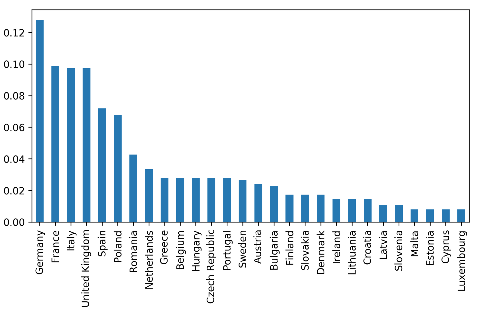
Here’s the distribution of the country. This is a very imbalanced classification.
Comparing words vs chars
.tiny-code[
bow_pipe = make_pipeline(CountVectorizer(), LogisticRegressionCV())
cross_val_score(bow_pipe, text_mem_train, y_mem_train, scoring='f1_macro')
array([ 0.231, 0.241, 0.236, 0.28 , 0.254])
char_pipe = make_pipeline(CountVectorizer(analyzer="char_wb"), LogisticRegressionCV())
cross_val_score(char_pipe, text_mem_train, y_mem_train, scoring='f1_macro')
array([ 0.452, 0.459, 0.341, 0.469, 0.418])
]
I can try to do either with word or character n-gram.
Using an f1 macro, I don’t get a good f1 score. If I use character n-grams, it’s not super great but it’s still quite a lot better than if we look at the words because I don’t need to learn new digital names.
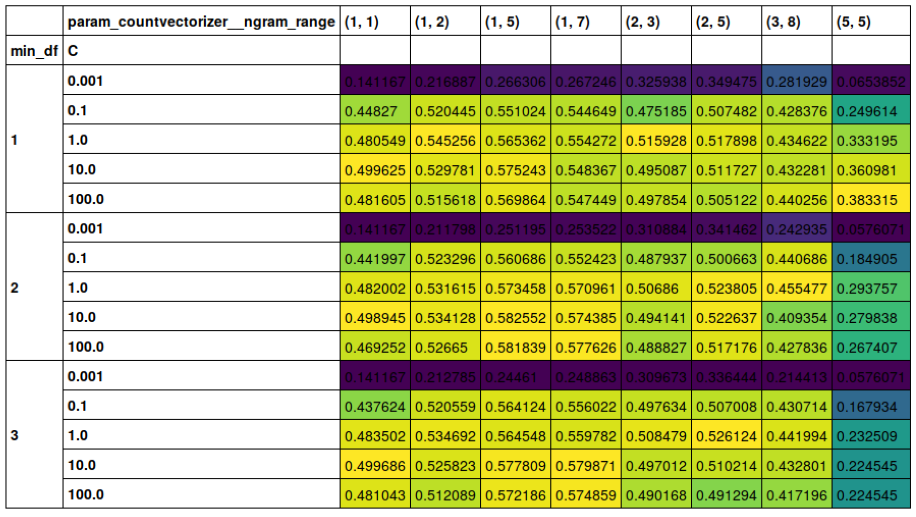
Grid-search parameters
.tiny-code[
from sklearn.model_selection import GridSearchCV
from sklearn.linear_model import LogisticRegression
from sklearn.preprocessing import Normalizer

param_grid = {"logisticregression__C": [100, 10, 1, 0.1, 0.001],
              "countvectorizer__ngram_range": [(1, 1), (1, 2), (1, 5), (1, 7),
                                               (2, 3), (2, 5), (3, 8), (5, 5)],
              "countvectorizer__min_df": [1, 2, 3],
              "normalizer": [None, Normalizer()]
             }
grid = GridSearchCV(make_pipeline(CountVectorizer(analyzer="char"), Normalizer(), LogisticRegression(),
                                  memory="cache_folder"),
                    param_grid=param_grid, cv=10, scoring="f1_macro"
                   )
grid.fit(text_mem_train, y_mem_train)
grid.best_score_
0.58255198397046815
grid.best_params_
{'countvectorizer__min_df': 2,
 'countvectorizer__ngram_range': (1, 5),
 'logisticregression__C': 10}
]
We can do a grid search, though that might take a while on the bigger dataset.
Things that you want to tune are a regularization of your models, I always use logistic regression CV to tune it internally. If I want to tune multiple things at once, I could use as a pipeline grid search.
Here, this is for character n-grams, but still, I might want to tune the n-gram range. If I was using bag of words, I might not look at sequences of 8 words because it will take very long to compute this and it’s probably not going to be useful.
Here, I’m using count vectorizer, but I could still normalize using the L2 normalizer.
Another thing, if you do something like this, you don’t want to fit each step of the pipeline every time. So some of these steps for the count vectorizer, if you have a big dataset, it might be pretty expensive and so you don’t want to refit this again, just because you’re plugged in the normalizer or just because you changed the C parameter in the logistic regression.
Make pipeline has a parameter called memory that allows you to cash the results. So you just have to give it a non-empty string and it’ll use that as the full name to catch the results. If there’s no catch eviction, at some point you need to delete it, or your hard drive will run full.
Here, you can see that after tuning everything, I actually get a result that’s much better than what I had before. So before I had an f1 macro of 0.45 and now I have 0.58.
So min_df=2 and ngram_range: (1,5) and c=10 gives the best results.
Small dataset, makes grid-search faster! (less reliable)
.center[
 ]
]
Here, I used pivot tables and Pandas to look into the effect of the different parameters.
Other features
Length of text
Number of out-of-vocabularly words
Presence / frequency of ALL CAPS
Punctuation…!? (somewhat captured by char ngrams)
Sentiment words (good vs bad)
Whatever makes sense for the task!
There are other kinds of features that you might want to look into.
There are actual collections of positive-negative words that you can download and you can check how many positive words are in this, how many negative words are in this. So basically, the model can share information about how important these words are because a particularly positive word might appear only very infrequently in your dataset but you can still learn that positive word means good.
Bag of words is a pretty good baseline. It’s a very simple approach and often gives reasonable results.
Large Scale Text Vectorization
The last thing I want to mention is how you can scale this up for really large scale stuff.
Basically just a very slight modification. So for example, if you want to use training a model on the Twitter stream, which has tweets coming in all the time, this has a couple of problems.
You don’t want to store all the data
Your vocabulary might shift over time. You might not be able to store the whole vocabulary, because the whole vocabulary of what everybody says on Twitter is very large.
There’s a trick which allows you to get away without building a vocabulary.
.center[
]
This is what we did before. We tokenize the string, split onto words, build a vocabulary and then built a sparse matrix representation. Now we can replace this vocabulary with just a hash function.
.center[
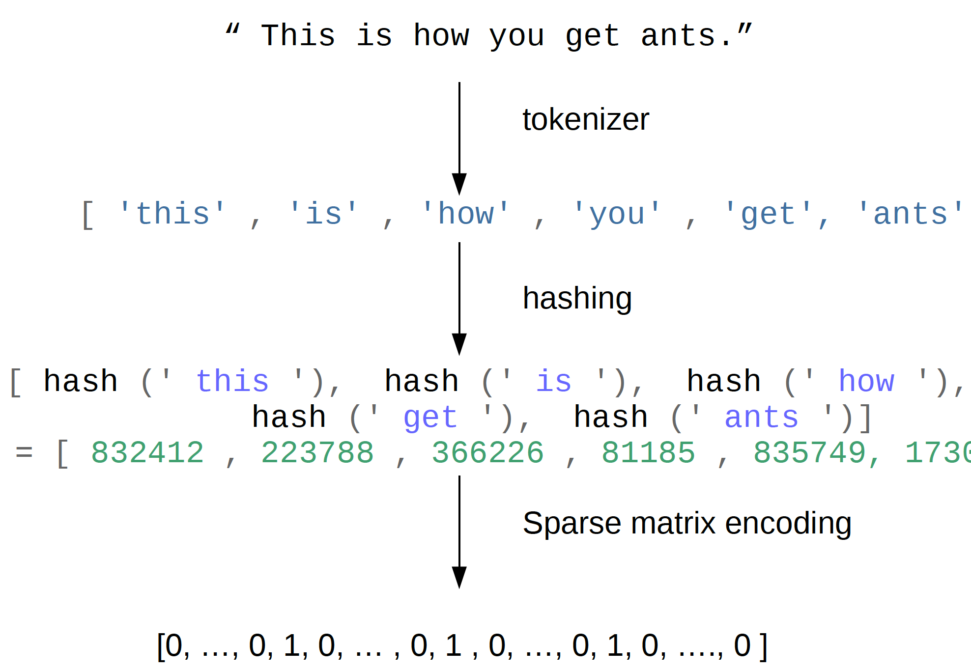 ]
]
And we can use any string hash function, that computes half of the token, then we represent this token just by its hash number.
Here, I used a hash method. This just hashes to 832,412 and so this is the number of the feature. Then I can use these as indices into my sparse matrix encoding. So now I need a hash function with some upper limits, let’s say 1 billion or something, and as I get a feature vector of length 1 billion. And then I can use these hashes as indices into this feature vector.
So I don’t need to build a vocabulary which is pretty nice.
Trade-offs
.left-column[ Pro:
Fast
Works for streaming data
Low memory footprint ] .right-column[ Con:
Can’t interpret results
Hard to debug
(collisions are not a problem for model accuracy)
]
Here are pros and cons listed.
It’s hard to interpret the results because now you have like a feature vector of size million, but you don’t know what the features correspond to. Previously we had a vocabulary and we could say feature 3 corresponds to X and now we don’t know what it is.
You could try to store the correspondences but that would sort of remove all the benefits. So that makes it kind of hard to debug.
There can be hash collisions, which make it harder to interpret. 2 tokens can hash to the same index. In practice, that’s not really a problem for accuracy. But it’s a problem for interpretability because you can’t undo the hash function so you don’t know why your model learned the thing it learned. But if you have really big text data or streaming setting, this is a quite simple and effective method.
Near drop-in replacement
.smallest[
Careful: Uses l2 normalization by default! ]
.tiny-code[
from sklearn.feature_extraction.text import HashingVectorizer
hv = HashingVectorizer()
X_train = hv.transform(text_train)
X_val = hv.transform(text_val)
lr.score(X_val, y_val)
from sklearn.feature_extraction.text import HashingVectorizer
hv = HashingVectorizer()
X_train = hv.transform(text_train)
X_val = hv.transform(text_val)
X_train.shape
(18750, 1048576)
lr = LogisticRegressionCV().fit(X_train, y_train)
lr.score(X_val, y_val)
]
This is a drop-in replacement for count vectorizer. It’s the hashing vectorizer. Here, you can see by default, it actually uses a hash base of about a million.
The result was about the same. It can be faster, and you get away without storing the vocabulary
Other libraries
LSA & Topic Models
04/13/20
Andreas C. Müller
Today, I’m going to talk about Latent Semantic Analysis and topic models, and a bit of Non-negative matrix factorization. The overarching theme is extracting information from text corpuses in an unsupervised way.
FIXME How to apply LDA (and NMF?) to test-data FIXME WHY / How FIXME steal from Tim Hoppers talk!! https://www.youtube.com/watch?v=_R66X_udxZQ FIXME do MCMC LDA (code)? FIXME explain MCMC? FIXME classification with logisticregressioncv instead of fixed C? FIXME preprocessing for LDA: mention no tfidf. FIXME Classification with NMF. FIXME Classification with LDA vs LSA? FIXME add non-negative constraint on NMF to objective slide?
Beyond Bags of Words
Limitations of bag of words:
Semantics of words not captured
Synonymous words not represented
Very distributed representation of documents
One possible reason to do this is that you want to get a representation of your text data that’s more semantic.
In bag of words, the semantics of the words are not really captured at all. Synonymous words are not represented, if you use a synonym it will be like a completely different feature and will have nothing to do with another feature. The representation is very distributed, you have hundreds of thousands of features and it’s kind of hard to reason about such a long vector sometimes, in particular, if you have longer documents.
Today, we’re going to talk about classical unsupervised methods. And next time, we’re going to talk about word vectors and word embedding, which also tries to solve the same problem of getting more semantically meaningful representations for text data.
Topic Models
Next, I want to talk a little bit about models that are somewhat more specific to the text data, or that allows us maybe to interpret the text data a little bit more clearly.
The idea of topic models is basically that each document is created as a mixture of topics. Each topic is a distribution over words. And we want to learn the topics that are relevant to our corpus and which of these topics contribute to each individual document.
Topics could be the genre of movie, or the sentiment, or the comment writer sophistication, or whether English is their native language or so on. And so each of them is would be topics. So the topic is not necessarily sorted of semantic topic, but something that influences the choice of vocabulary for a given document.
For each document, you assume that several of these topics are active and others are not and they have very varying importance. So movies could be mixtures of different genres and then they could have words from multiple genres.
Motivation
Each document is created as a mixture of topics
Topics are distributions over words
Learn topics and composition of documents simultaneously
Unsupervised (and possibly ill-defined)
This is an unsupervised task, so it’s probably ill-defined and so results are open to interpretation, and also depend on how exactly you formulate the task.
#Matrix Factorization
.center[
 ]
]
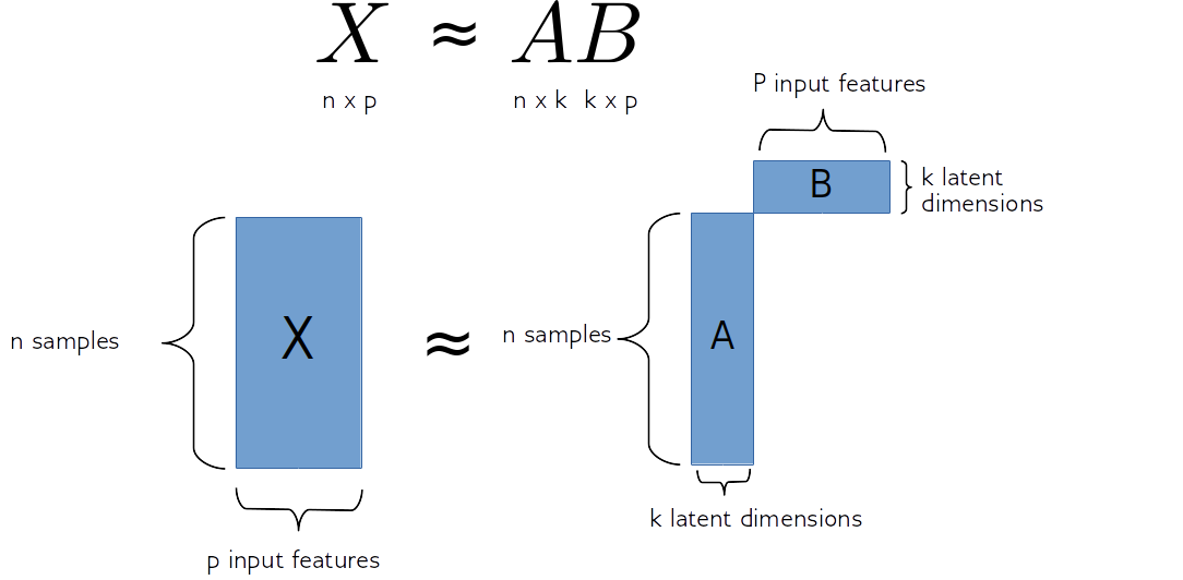
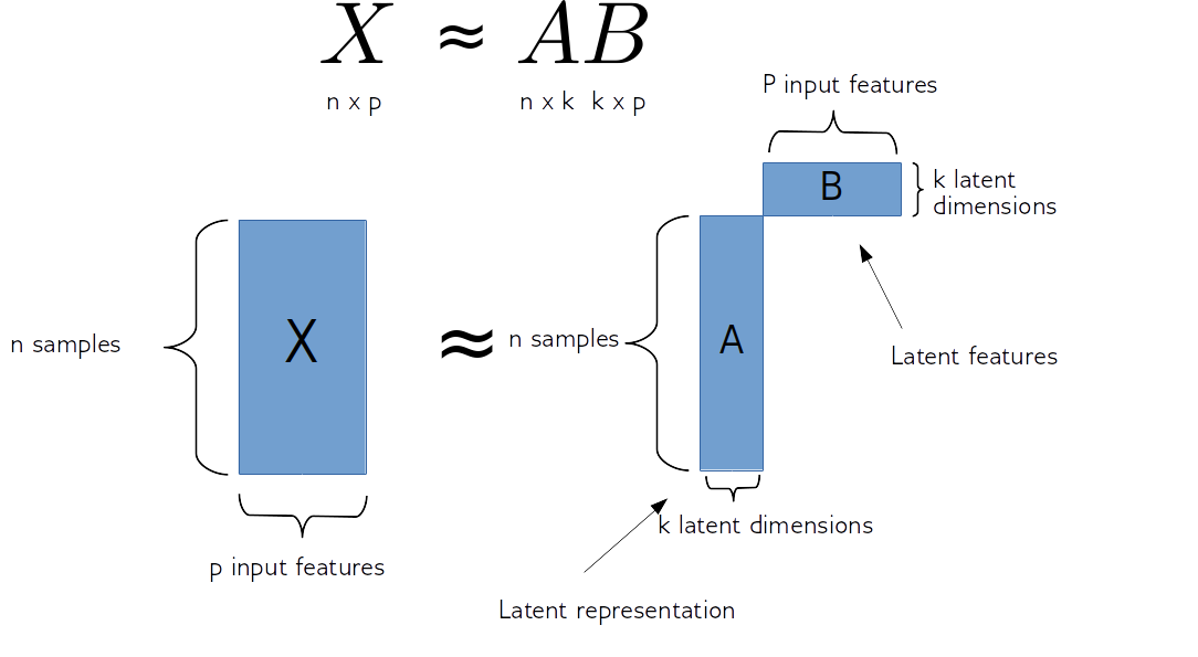
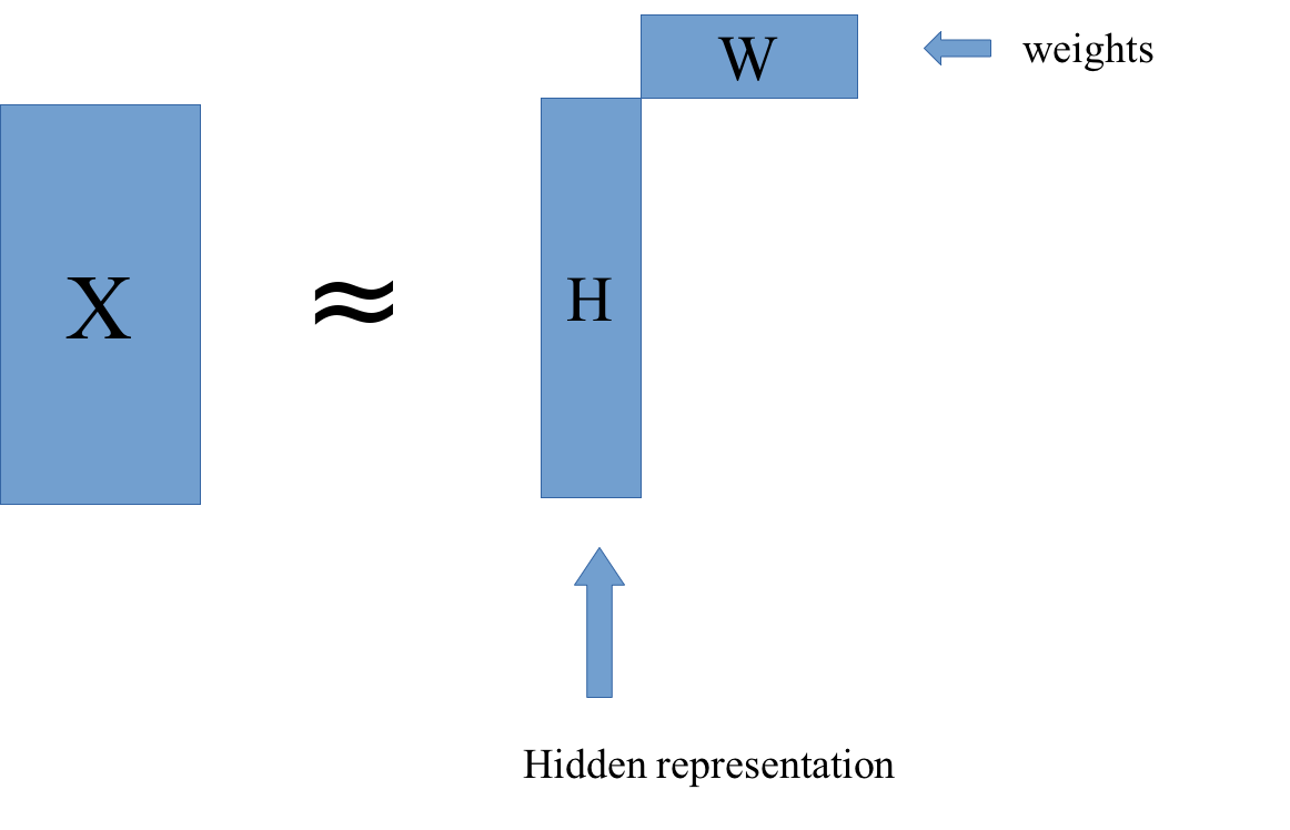
So matrix factorization algorithm works like this. We have our data matrix, X, which is number of samples times number of features. And we want to factor it into two matrices, A and B.
A is number of samples times k and B is k times number of features.
If we do this in some way, we get for each sample, a new representation in k-dimensional, each row of k will correspond to one sample and the columns of B will correspond to the input features. So they encode how the entries of A correspond to the original data. Often this is called latent representation. So, these new features here in A, somehow represent the rows of X and the features are encoded in B.
#Matrix Factorization
.center[
 ]
sklearn speak:
]
sklearn speak: A = mf.transform(X)
#PCA
.center[
 ]
]
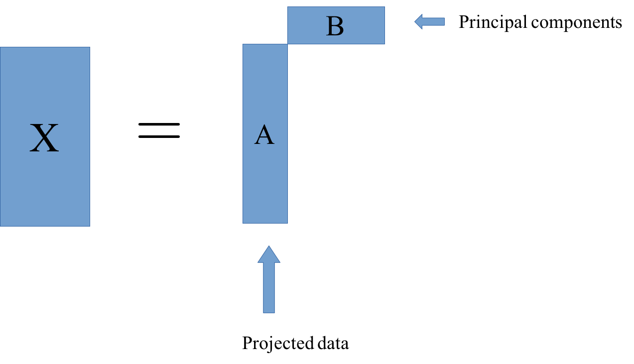
The one example of this that we already saw is principal component analysis. In PCA, B was basically the rotation and then a projection. And A is just the projection of X.
This is just one particular factorization you can do. I have the sign equal, but usually, more generally, you’re trying to find matrixes A and B so that this is as close to equal as possible.
In particular, for PCA, what we’re trying to do is we try to find matrices A and B so that the rows of B are orthogonal, and we restrict the rank of k. K would be the number of components and we get PCA, if we restrict the columns of B to be orthogonal, then the product of matrixes A and B is most close to X in the least square sense is the principal component analysis.
Latent Semantic Analysis (LSA)
Reduce dimensionality of data.
Can’t use PCA: can’t subtract the mean (sparse data)
Instead of PCA: Just do SVD, truncate.
“Semantic” features, dense representation.
Easy to compute - convex optimization
LSA is basically just the same as PCA. The idea is to reduce the dimensionality of the data to some semantically meaningful components. The thing is, we can’t easily do PCA here, because we can’t remove the mean. Remember, this is a sparse dataset and so the zero is sort of meaningful and if we shift the zero, like by trying to subtract the mean, we will get a density dataset that won’t have many zeros anymore and so we won’t be able to even store it.
There are ways to still compute PCA without explicitly creating a big dense matrix, but in the traditional LSA, we just ignore that and do a singular value decomposition of the data. This is exactly the same computation as PCA, only, we don’t subtract the mean.
This is very easy to compute. You can do the SVD very easily. And there’s a unique solution that you can compute. And then you have something that’s like a dense representation of the data and hopefully, it’s semantic in some way.
As with all unsupervised methods, this can be hit or miss a little bit.
LSA with Truncated SVD
.smaller[
from sklearn.feature_extraction.text import CountVectorizer
vect = CountVectorizer(stop_words="english", min_df=4)
X_train = vect.fit_transform(text_train)
X_train.shape
(25000, 30462)
from sklearn.decomposition import TruncatedSVD
lsa = TruncatedSVD(n_components=100)
X_lsa = lsa.fit_transform(X_train)
lsa.components_.shape
(100, 30462)
]
So the way to do this with scikit-learn is with truncated SVD. Truncated SVD is basically the implementation of PCA that doesn’t subtract the mean. We didn’t call it LSA, because if you do this in the context of text processing, you can do this whenever you have a sparse dataset, you would want to do something like PCA but it’s sparse, then you can use the truncated SVD.
Here, I’m just using the training set, 25,000 documents, I removed the stop words, and I set min_df=4.
So basically, I removed the most common words, which are stop words, and I removed the very infrequent words. So I have a more reasonably sized vocabulary. And then I did a truncated SVD and extract 100 components. And so the components I extracted, are 100 X number of features. So I have 100 vectors, where each feature corresponds to one of the words in the vocabulary.
.smaller[
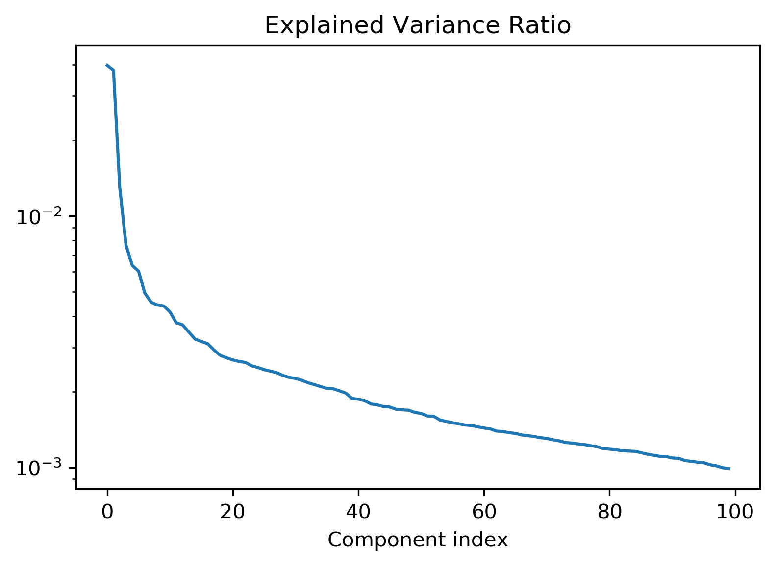
plt.semilogy(lsa.explained_variance_ratio_)
]
.center[
 ]
]
As we saw with PCA, we can look at the explained variance ratio.
Here’s is a semi-log scale. And you can see that the first one or two explain a lot and then rapidly decreases. A lot is captured in the first 10, and then it goes down.
But still at 100, there’s still a lot of variances left, so it’ll just probably go down logarithmically as it goes on. We can also look at the eigenvectors with the highest singular values.
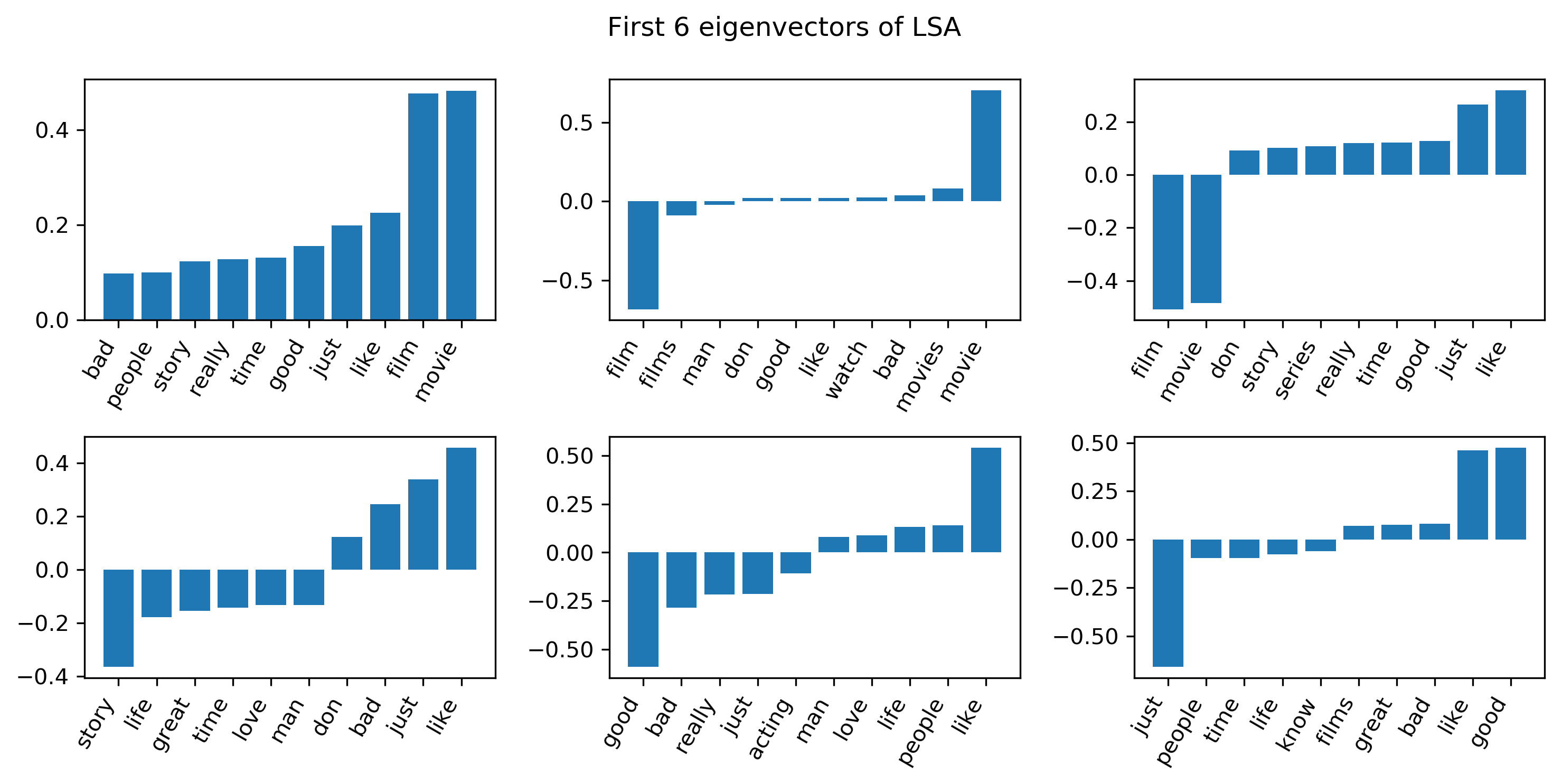
First Six eigenvectors
.center[
 ]
]
Here are the 6 first eigenvectors. I’m showing only the entries that have the largest magnitude, either positive or negative.
I’m showing the 10 largest magnitudes entries of each of the eigenvectors. So again, keep in mind that the sign doesn’t really mean anything, since its eigenvalues, but sort of the relative sign means something.
So the first one is sort of what you would usually get. They’re all positive because all entries in the data matrix are positive since its bag of words. This is sort of, in a sense, just translating into the middle of the data, somewhat similar to trying to model the mean. ‘Movie’ and ‘film’ are obviously the most common words.
The second eigenvector is whether someone uses the word ‘movies’ or ‘films’. You can see that either someone uses ‘film’ and ‘films’ or ‘movie’ and ‘movies’. Basically, people don’t usually use both of them in the same comment. It is just interesting that this is the one of the largest components of variances, whether a person uses this one word or this other word that is completely synonymous.
Points in direction of mean
Scale before LSA
from sklearn.preprocessing import MaxAbsScaler
scaler = MaxAbsScaler()
X_scaled = scaler.fit_transform(X_train)

lsa_scaled = TruncatedSVD(n_components=100)
X_lsa_scaled = lsa_scaled.fit_transform(X_scaled)
There are 2 things that you can do, you can normalize for the length of the document, or you can scale so that all the features are on the same scale.
MaxAbsScaler performs the same way as a standard scaler, only it doesn’t subtract the mean. So it just scales everything to have the same maximum absolute value. And so in this sense, I’m basically scaling down film and movie to have the same importance as the other words. I can also normalize and get rid of the length of the document. But I don’t think it actually had an effect here. And then I can compute the same thing.
“Movie” and “Film” were dominating first couple of components. Try to get rid of that effect.
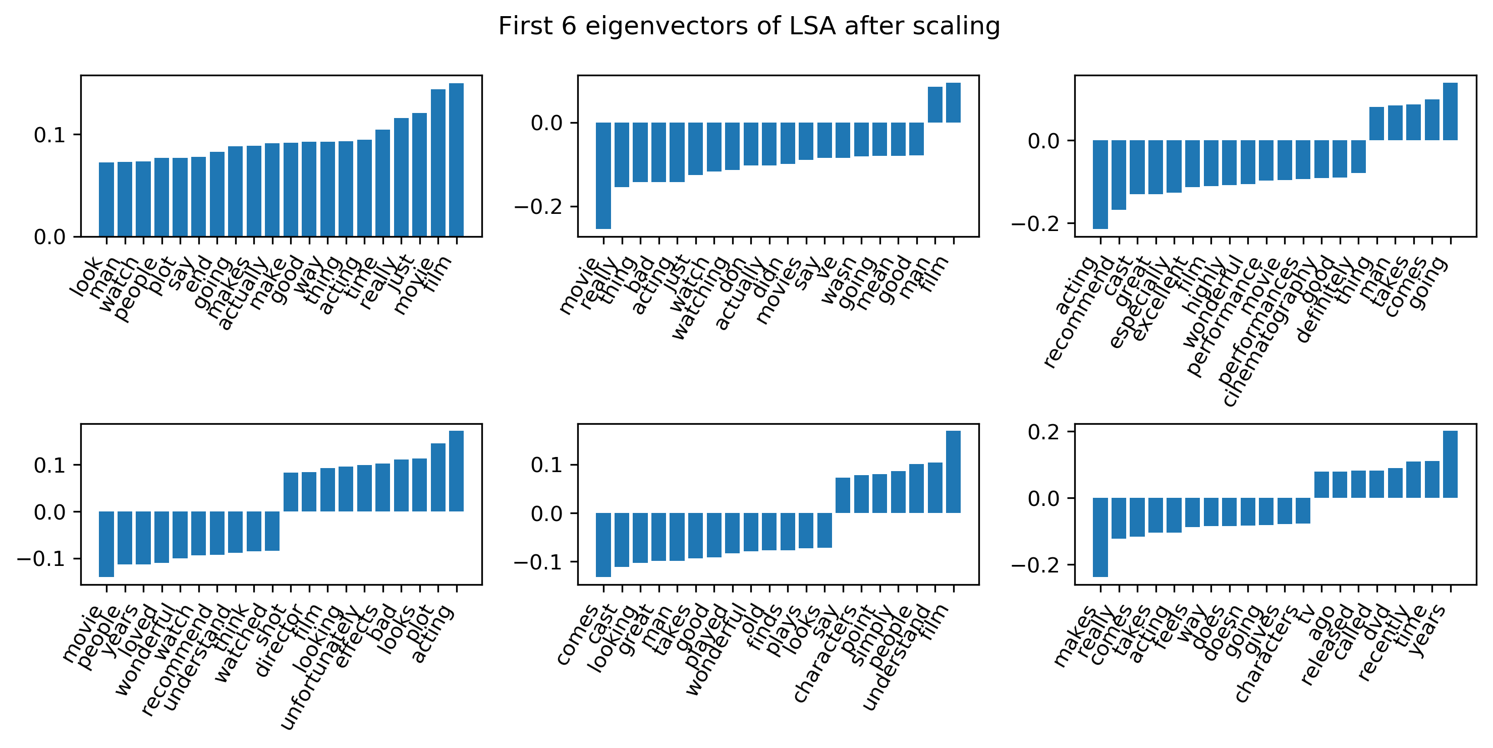
Eigenvectors after scaling
.center[
 ]
]
This is the first six eigenvectors of LSA after scaling. The first one still points towards the direction of the mean. So I found some components like the third one here, which are interesting because I interpreted this as like a writer sophistication. So there are some people that use a lot of very short words and some people use a lot of very long words. So people that use words like ‘cinematography’ also use words like ‘performance’ and ‘excellent’. This also comes out from some of the other methods.
And so I looked at a couple of these components and it turned out that the component 1 and the component 3 are actually related to the good and bad review.
Movie and film still important, but not that dominant any more.
Some Components Capture Sentiment
.smallest[
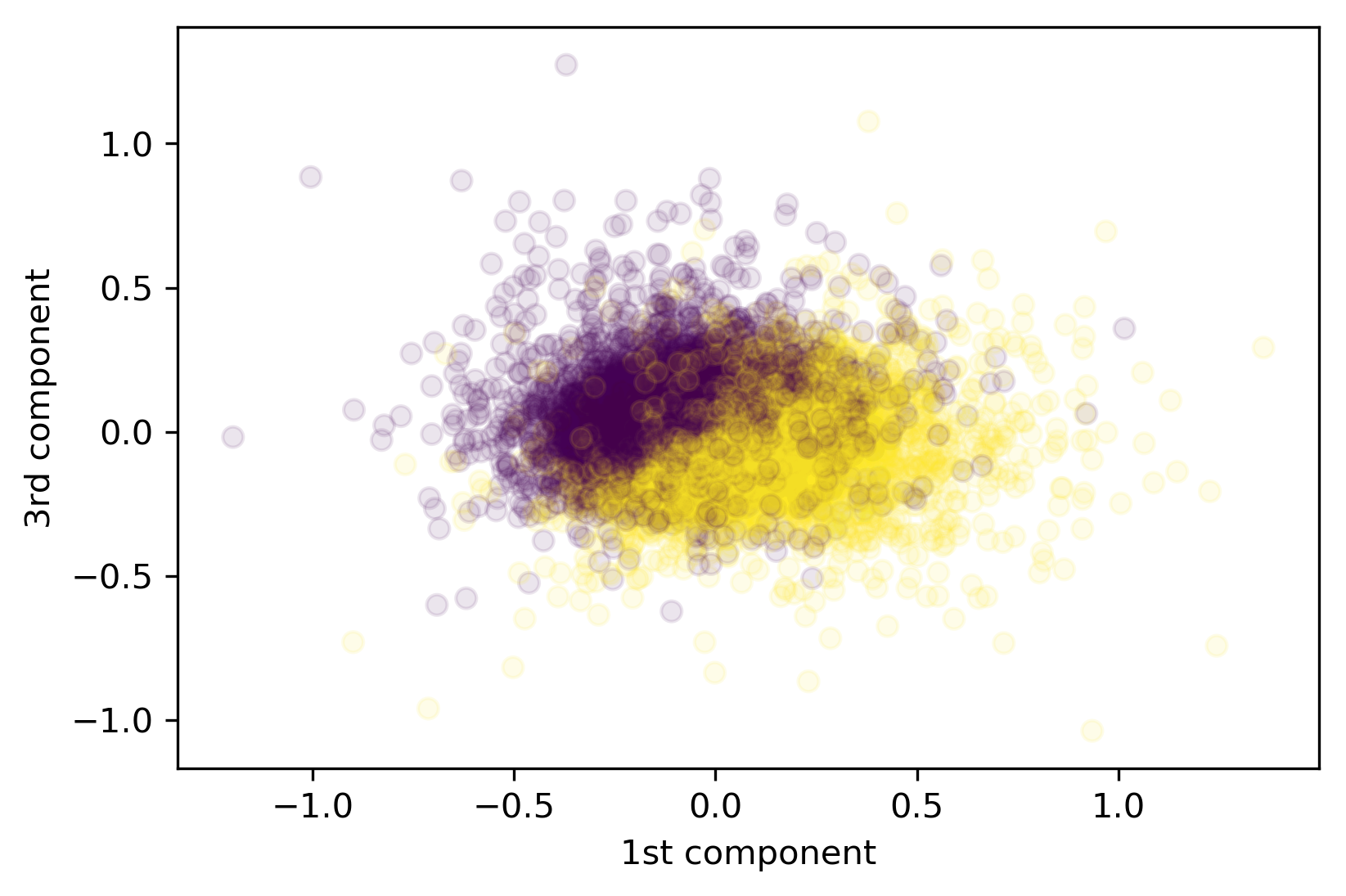
plt.scatter(X_lsa_scaled[:, 1], X_lsa_scaled[:, 3], alpha=.1, c=y_train)
]
.center[
 ]
]
.smallest[
lr_lsa = LogisticRegression(C=100).fit(X_lsa_scaled[:, :10], y_train)
lr_lsa.score(X_test_lsa_scaled[:, :10], y_test)```
0.827
```python
lr_lsa.score(X_lsa_scaled[:, :10], y_train)
0.827
]
This scatter plot is positive reviews versus negative reviews. Some of the components actually capture the semantic attributes we are interested in.
It was completely unsupervised, we didn’t put that in and this is just a bunch of movie reviews. But these two components, actually, seem to be pretty related to the sentiment of the comment writer.
I also run a logistic regression on 10 components and it was at 83% accuracy.
I thought that was actually pretty good. It was 88% using the bag of word representation. So you got 88% if you used 30,000 dimensions, and you get 83% if you used 10 dimensions. So it is completely unsupervised compression of the data. So it’s not as good as the original data set but if you take 100 components you recover the same accuracy.
So these components definitely capture something that’s semantic, and it allows us to classify even if we use lower dimensional representation.
Not competitive but reasonable with just 10 components
NMF for topic models
.center[
 ]
]
The first model I want to use for this is NMF.
In NMF, remember, we have a data matrix, X, which is now our large sparse matrix of word counts and we factorize this into HxW, H is the hidden or latent representation, and W represents the weights.
NMF Loss and algorithm
Frobenius loss / squared loss ($ Y = H W$):
Kulback-Leibler (KL) divergence: \($ l_{\text{KL}}(X, Y) = \sum_{i,j} X_{ij} \log\left(\frac{X_{ij}}{Y_{ij}}\right) - X_{ij} + Y_{ij}\)$
s.t. H, W all entries positive
optimization :
Convex in either W or H, not both.
Randomly initialize (PCA?)
Iteratively update W and H (block coordinate descent)
–
Transforming data:
Given new data
X_test, fixedW, computingHrequires optimization.
In literature: often everything transposed
You want X to be close to HxW, that’s the whole goal. There are 2 common ways in which people measure this.
The first one at the top is called x norm, it’s just least squares basically. So you look at the least squares difference element-wise between the entries in the X and the entries in the product, 〖HW〗_ij. This one is the mostly common used one and also the default in scikit-learn.
The bottom one is the one which was originally proposed, which is basically, a version of the KDE, which is usually a measure that finds similarities between distributions. But here, it’s applied basically to element-wise entries of this matrix. The authors use that because then they could drive nice ways to minimize this.
Minimizing either of these is not convex but if you hold one of the two fixes, then minimizing the other one is convex. So you usually iterate doing either gradient descent or coordinate descent on H and then doing it on W, then you’re iterate between the two.
NMF for topic models
.center[
 ]
]
When applying this to text, the rows of X, corresponds to movie reviews, the columns of X correspond to words. So that means the rows of H, correspond to documents, and the columns of H correspond to the importance of a given topic for a given document. The rows in W corresponds to topics, one row in W is lengths of vocabulary that states the words that are important for a particular topic. So you might have a component with like horror, scary, monster and so on.
If the first topic is about horror movies, and the first movie is a horror movie, then it would be a large first component. Since everything is positive, and so the additive components are added together. That possibly makes it a little bit more interpretable.
Each row of W corresponds to one “topic”
NMF on Scaled Data
.smallest[
nmf_scale = NMF(n_components=100, verbose=10, tol=0.01)
nmf_scale.fit(X_scaled)
]
.center[
 ]
]
Sorted by “most active” components
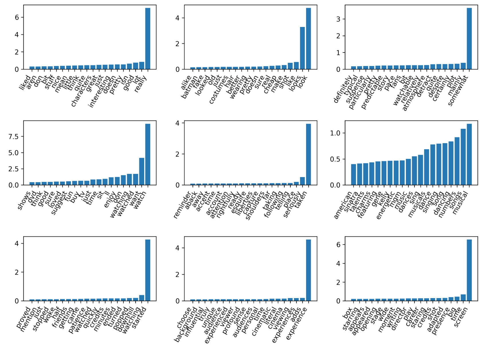
NMF, as I said, is an iterative optimization so this runs way longer than the LSA.
Q: What’s the variable ’tol’ do? A: It’s stopping tolerance.
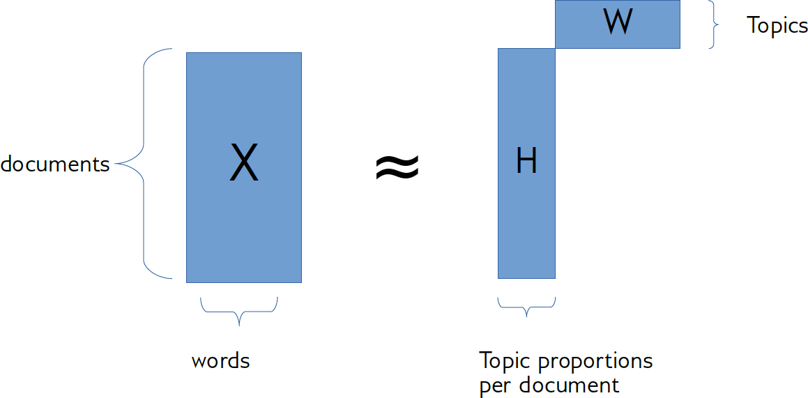
These are subsets of the columns of W. I’m visualizing the rows of W and I’m only looking at the ones that have large absolute values. So the Y values are the weight that this word has inside this topic. So the word ‘really’ has the weight of 7 in this first topic.
So obviously, they have entries for all words, but I didn’t put in a penalty so that they’re sparse. So they’ll have non-zero entries for all words, but sort of the interesting ones are the big ones.
The way that I picked these 9 components here out of the 100 components was the ones that have the highest activation in X. I, then realize it might not be the most interesting thing. Might be more interesting to look at the ones that are less peaked.
If you look at more components, you’ll find other genre-specific components.
One of the things you can do with this is you can find genre specific reviews by looking at the component that corresponds to it.
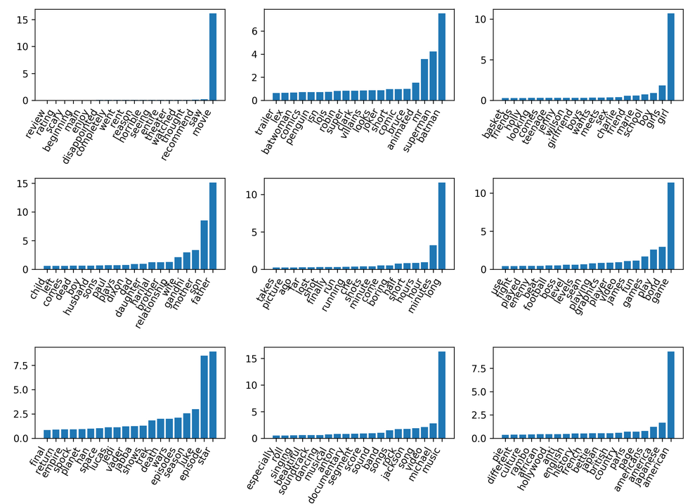
NMF with tfidf
You can also run this on TF-IDF. Again, results are somewhat similar to before. The top-ranked components are now different. It really only makes sense if you look at all 100 components, but it’s very hard to do. So I picked out just a couple.
This was with a 100 components. That said, if you use fewer components, you get something that is much more general.
NMF with tfidf and 10 components
.center[
 ]
]
This is using 9 components. The first one, probably kind of models the mean and points in the center.
Q: is the task here still to classify between good and bad reviews?
The application of that I had in the back of my head is I’m interested in the reviews, good or bad, but this is all completely unsupervised. So I never put in anything about these two classes even existing. This is just trying to help me understand corpus overall.
The main things that I found so far are that it finds things that are genre specific, some of them are very specific, like Star Wars and DC comics, some of them are less specific like horror movies, but then it finds some that are about sentiments.
The reason why I call these topics is since they are additive. And so maybe someone would argue that this is not really a topic model, because it’s not technically a topic perfect model but it does exactly the same as a topic model does. It does a positive decomposition. I think that’s easier to interpret in this context. Because what does it mean for a document to be not about horror movies.
Less number of components will give you more generic things. If you use more number of components, there might be generic components. If you want to force them to be generic, you can use fewer components. Using fewer components definitely makes it easy to look at them.
A friend of mine who is an expert on topic models told me to always use thousands of components, and then go through all of them and see if something’s interesting.
#Latent Dirichlet Allocation
(the other LDA)
(Not Linear Discriminant Analysis)
Next thing I want to talk about is LDA. We are going from simple models to more complex model.
What people think about if they hear topic model is usually LDA. Dave Blei in the sets department invented LDA. This is like an incredibly popular model right now.
The LDA Model
.center[
 ]
.smallest[
(stolen from Dave and John)
]
]
.smallest[
(stolen from Dave and John)
]
This a probabilistic generative model. The idea is you write down a generative process of how each document is created. This is similar to mixture models where basically, for each point you want to create, you picked one of the Gaussians and then you sample from it. That’s how we create points in this distribution.
Similarly, in the LDA model, let’s say, you’re given some topics and these topics have, like word importance. Given the topics, the way that you generate a document would be, first, you draw which of these topics are important, and how important are they?
Each document is a mixture of topics and then for each word, you decide which of these topics to you want to draw a word from. And then you draw a word from that topic, according to the word importance.
This is clearly not really how text is generated but it’s sort of reasonable proxy. This is based on the bag of word model so it only looks at word counts. It doesn’t do that context at all. You could do it on bigrams, but that’s not what people usually do.
The idea is how likely is it that a word appears in this document and basically, for each word individually, you pick a topic, and then you generate a word from this topic and in the end, you end up with a big bag of word representation. The idea is that this a generative process, given corpus of documents, can I actually do inference in this? Can I find out what were the topics that generated this model? And what are the topic proportions for each of the documents? And what are the word assignments?
So basically, you write down this generative process and then given your documents, you’re trying to invert it and figure out what were the topics.
Generative probabilistic model (similar to mixture model)
Bayesian graphical model
Learning is probabilistic inference
Non-convex optimization (even harder than mixture models)
.center[
 ]
]
.smallest[
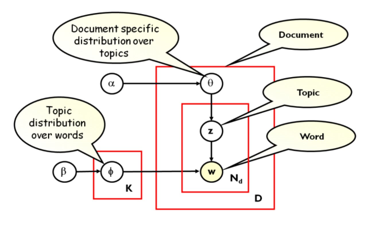
For each topic \(k\), draw \(\phi_k \sim \text{Dirichlet}(\beta), k = 1 ... K\)
For each document \(d\) draw \(\theta_d \sim \text{Dirichlet}(\alpha), d = 1 ... D\)
For each word \(i\) in document \(d\):
Draw a topic index \(z_{di} \sim \text{Multinomial}(\theta_d)\)
Draw the observed word \(w_{ij} \sim \text{Multinomial}(\phi_z)\)
(taken from Yang Ruan, Changsi An (http://salsahpc.indiana.edu/b649proj/proj3.html) ]
You can write down this generative model in flight notations. I don’t think we looked at the plate notation yet because I don’t find it very helpful.
So this is a depiction of the graphical model where basically, each of these circles is a variable. And these red things are called plates and they mean a variable is duplicated.
So here, there are 2 parameters you specified beforehand, which are the hyperparameters, Alpha and Beta.
Then there are K topics, I fixed the number of topics and I call them K. And for each topic, I have a distribution over words, like how important is each word in each topic. Then D goes over documents. So for each document, I have a distribution over the topics that states that a particular document is so much about this topic, and so much about another topic.
So for each document, I have a vector that tells me the topic proportions. Finally, inside the document, for each word I have a variable, that tells me which topic the word belongs to and then given the topic, what is the word.
Here, this outer plate is replicated along all the documents and then inside each document, for each word, there’s the inner plate.
But the only thing that I actually observe is basically the W, which is the word count. So I observed which words appeared in these documents. I also set alpha and beta as some prior parameters usually.
What I want to find out is the topic distribution over words and the documents specific distributions over topics. So I want to know what the topics are and what topics are a given document about.
This is very similar to the thing that we had in NMF.
The flight notation graph can be read as A) The generative process or B) Dependency structure in the probability distribution.
So basically, the distribution that you can easily think of is like, what should the work distribution be? And so the word, I choose it from a discreet of distribution, like given a particular topic, I take the distribution of words in this topic and I pick from that distribution.
So this is a categorical distribution where you say, under this distribution, each word is so and so likely. So this multinomial distribution, this is how I pick a word given a topic.
But the distribution in this is Dirichlet data distributions.
Basically, you want the distribution over distribution, you want the distribution where the outcome is multinomial distribution, and for the W, I want multinomial distributions and so the pi, the outcome of drawing there, needs to be multinomial distribution.
The national prior over things that give me multinomial distributions is called Dirichlet.
K topics = multinomial distributions over words
“mixture weights” for each document:
How important is each topic for this document
Each document contains multiple topics!
Multinomial
.smaller[It models the probability of counts for rolling a k-sided die n times.] .quote_author[wikipedia]
–
Dirichlet
if \(p(x|\theta)\) is multimnomial (discrete distribution), then \(p(\theta) = \text{Dirichlet}(...)\) is a conjugate prior.
This is how it looks in formula. For multinomial, let’s say I draw n words from a multinomial. There are k possible words, I draw n, so I draw the same word multiple times, and the probability of drawing a particular word is P1 to Pk. So then the probability of a specific draw is P1 to X1, and so on from Pk to the Xk and then normalized.
Dirichlet is basically the same, only the other way around. You can see that here, the Ps in multicultural distribution become the Xs in Dirichlet distribution. Dirichlet looks exactly the same. Only now, you have a distribution over these base probabilities.
That makes it very easy to include the data into the prior information and compute the posterior.
Conjugate Prior
Prior is called “conjugate” of the posterior has the same form as prior \($ P(\theta | x) = \frac{p(x | \theta)p(\theta)}{\int_{}^{} p(x | \theta^\prime)p(\theta^\prime)d\theta^\prime} $\)
The reason why we’re using generative prior is because of the conjugate prior of the multinomial distribution. Let’s say we have a prior over our word topic distribution and then we observe some words belonging to some of the topics, we have some evidence that these words are drawn from these topics and then we want to update our word topic prior, given the information that we saw.
p(x|θ) would be our multinomial distribution, meaning given the topic, what are the multinomial distribution. And basically, we want p(θ|x) to be easy to compute. And it’s easiest to compute if we use the conjugate prior here, because then posterior will have the same distribution as the prior.
Dirichlet Distributions
.left-column[ PDF: \(\qquad \frac{1}{B(\alpha)} \Pi_{i=1}^{K}{x_i^{\alpha_i - 1}}\) ]
.right-column[ Mean: \(\qquad E[X_i] = \frac{\alpha_i}{\sum_k{\alpha_k}}\) ]
.center[
 ]
]
Here are some examples in 3D. Dirichlet distribution is like a distribution over distributions. So a point drawn from Dirichlet distribution is a multinomial distribution.
So here, let’s say you have a multinomial with 3 variables, this lives inside the probability simplex in 3-dimensions. The dark blue sector is sort of the space all 3 numbers that sum up to one.
And so now you can try put a prior on this. So we want to distribution over the simplex of all 3 numbers that add up to 1. And so what we’re doing for LDA is usually, we make this sort of symmetric in all directions because we don’t really have a preference for like, saying one topic is more important than the other topic, that’s not our prior knowledge, because they are arbitrary.
It’s pretty likely that all the topics are equally important, that means I have put math only in the very center or I can say, I didn’t really know how important each of the topics is, and then you can get points at the corners, which means that each document can be about only a few topics. If you use this, then each document will be about many topics.
And similarly, these priors use both on the document topic distribution, and on the topic word distribution. So similarly, for each topic, you can have each topic being very broad.
So the third one means broad, you assign probability mass to most words. While the first one means you can assign probability mass only to a couple of the words.
.center[
]
.smallest[
For each topic \(k\), draw \(\phi_k \sim \text{Dirichlet}(\beta), k = 1 ... K\)
For each document \(d\) draw \(\theta_d \sim \text{Dirichlet}(\alpha), d = 1 ... D\)
For each word \(i\) in document \(d\):
Draw a topic index \(z_{di} \sim \text{Multinomial}(\theta_d)\)
Draw the observed word \(w_{ij} \sim \text{Multinomial}(\beta_z)\)
(taken from Yang Ruan, Changsi An (http://salsahpc.indiana.edu/b649proj/proj3.html) ]
Two Schools (of solvers)
.left-column[ Gibbs Sampling
Implements MCMC
Standard procedure for any probabilistic model
Very accuracte
Very slow
]
.right-column[
Variational Inference
Extension of expectation-maximization algorithm
Deterministic
fast(er)
Less accurate solutions
Championed by Dave Blei
]
There’s basically 2 schools of thought on how we can best solve this. These are ways to do inference and generalize the models.
Gibbs sampling is a form of MCMC, so it’s like a stochastic simulation. Basically, you simulate process going on for a long time, you keep sampling and in the end, you get as a stationary distribution, the real distribution that you’re interested in. This is very accurate. You can do this for any probabilistic model. But it’s very slow because you need to simulate the process of generating the data for a long until it lines up with what’s in the data. Gibbs sampling a form of sampling so it’s like a very random process.
The other one is variational inference. This is more from an optimization perspective. This is very similar to the expectation-maximization algorithm that’s used for GMMs, which is similar to that of the KMeans idea of alternating between assignment and maximization. This is a deterministic algorithm, it’s quite a bit faster than Gibbs sampling usually, but less accurate. The way that it does approximations is not entirely clear. This is used by Dave Blei all the time.
Pick a solver
“Small data” ( < = 10k? Documents):
Gibbs sampling (lda package, MALLET in Java)
“Medium data” ( < = 1M? Documents):
Variational Inference (scikit-learn default)
“Large Data” (>1M? Documents):
Stochastic Variational Inference
SVI allows online learning (partial_fit)
Tensorflow Probability https://www.tensorflow.org/probability
Tensor-flow based framework for stochastic variational inference.
Used to be Edward by Dustin Tran (Blei Lab)
Pick a solver depending on the amount of the documents you have.
Ida package (Python) and MALLET (Java) works well if you have very few documents. Otherwise, it gets too slow.
Variational inference or batch variational inference, which will be the default in scikit-learn in the future. Both are used on medium sized documents.
For large data, you can do stochastic variation inference, which is the current default in scikit-learn. But that’s sort of an approximation to the approximation. It’s something like doing stochastic gradient descent on the optimization variational inference.
Partial_fit can be used on streaming data.
If you’re more serious about this, look at the works of Dustin Tran. He created Edward, I think it’s now incorporated into TensorFlow. It’s a library for doing variational inference in all kinds of different graphical models with GPU acceleration.
Talking about SGD, maybe it’s good if have a lot of data, maybe it’s worth doing an approximation that allows you to use all the data, if the other option is to do something that’s fairly exact, but you have to subsample your data a lot, then that might give you worse results than just doing something that’s pretty bad.
SVI is maybe not the greatest optimizer but it allows you to use large amounts of data, and so in the end to get a better result.
Variational might be more sensitive to hyper parameters? Or give different results?
.smallest[
from sklearn.decomposition import LatentDirichletAllocation
lda = LatentDirichletAllocation(n_components=10, learning_method="batch")
X_lda = lda.fit_transform(X_train)
]
.center[
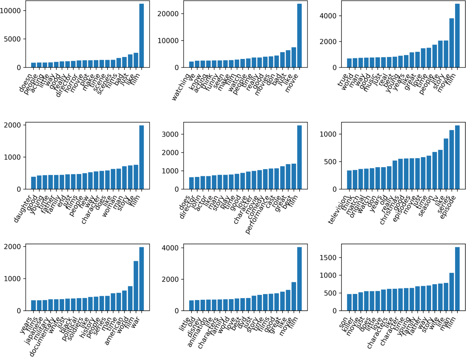 ]
]
Implementing in scikit-learn is pretty straightforward. The components are not ordered, and changing number of components changes everything. Here, I do learning_method=batch and the other one is learning_method=online, but since the dataset is not that big, it’ll just give me sort of worse results.
Everything is positive because these are now the word topic matrices. It tells me if I picked this topic, what’s the probability of each of these words and they’re actually on a log scale. They sum up to 1 in a sense. This is using 10 topics, so this is pretty generic.
Very generic, similar to NMF(n_components=10). TV Series, “family drama”, and “history / war” topics
.smallest[
lda100 = LatentDirichletAllocation(n_components=100, learning_method="batch")
X_lda100 = lda100.fit_transform(X_train)
]
.center[
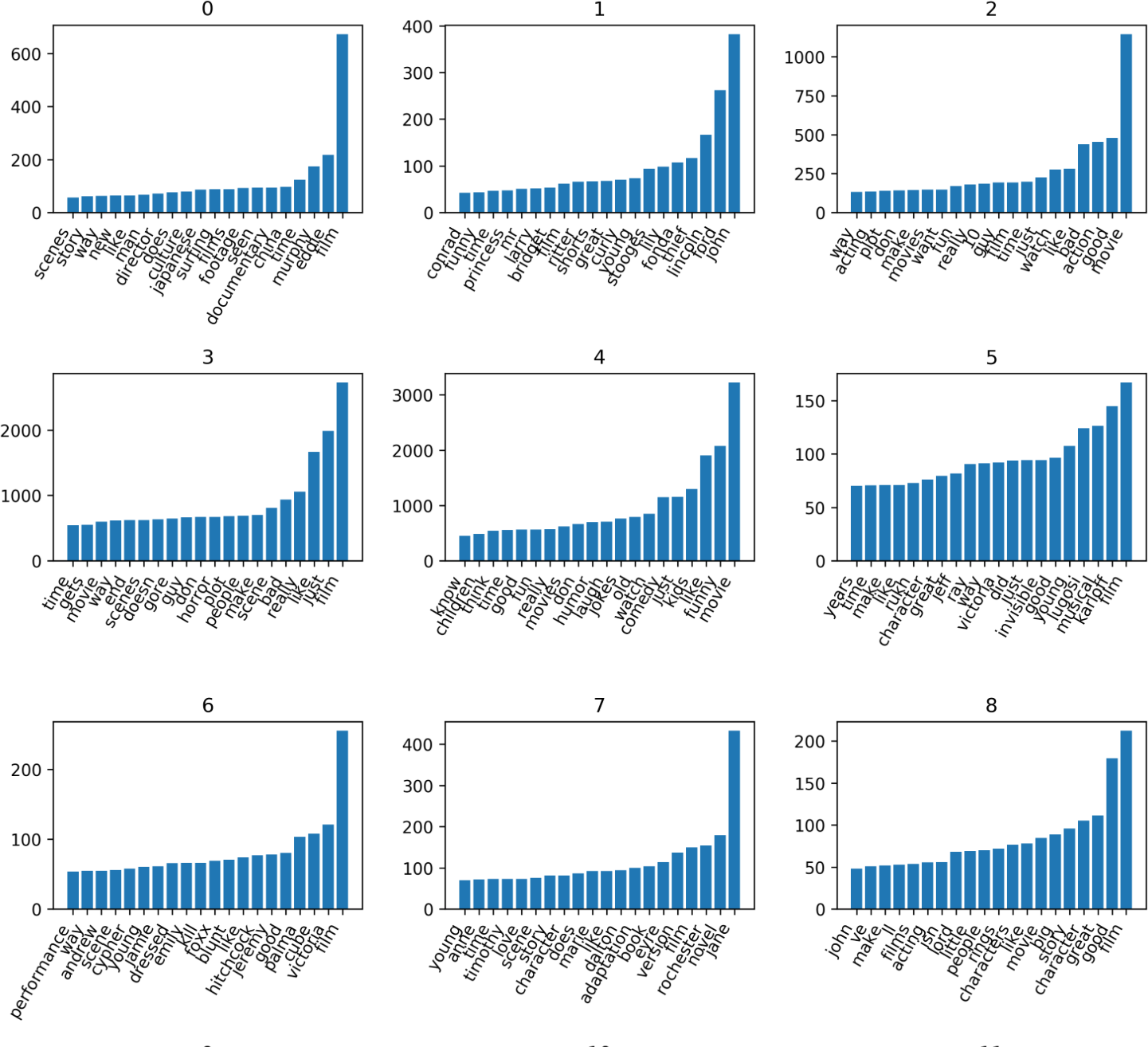 ]
]
This showing 9 out of 100 documents.
.center[
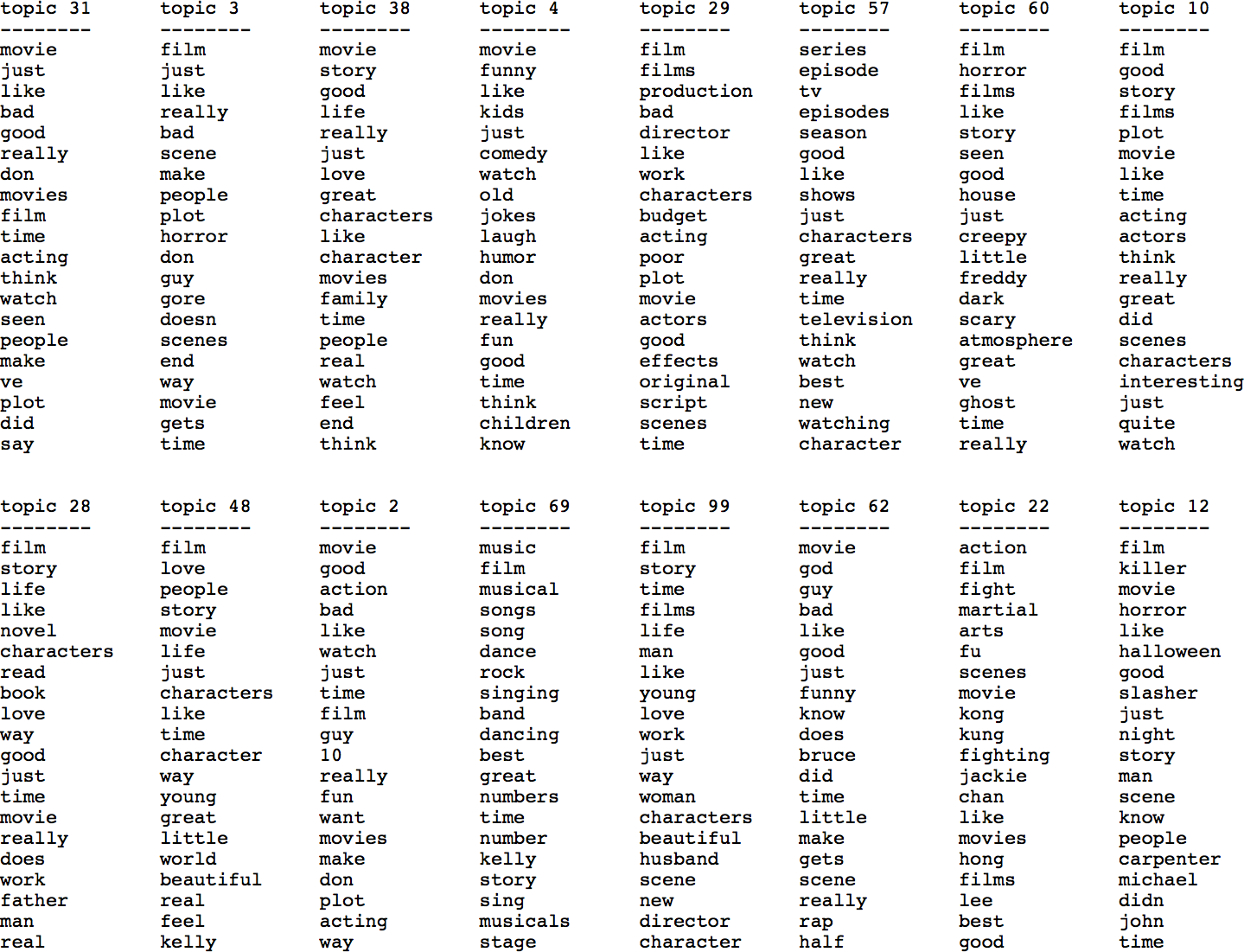 ]
]
Here, I picked out a couple of topics that I thought were interesting.
One thing that you can do is try to interpret this. You can use both this and NMF as a representation for classification, for example. There’s no guarantee that it’s a good representation, but it might be a better representation than the bag of words.
If you do the NMF with 100 components, you actually get a slightly better result than if you use just a bag of word vectors. Doing the NMF actually helps you to get some features that are semantic for the task of classifying good versus bad reviews.
Hyper-Parameters
\(\alpha\) (or \(\theta\)) = doc_topic_prior
\(\beta\) (or \(\eta\)) = topic_word_prior
Both dirichlet distributions
Large value \(\xrightarrow[]{}\) more dispersed
Small value \(\xrightarrow[]{}\) more concentrated
.center[
]
I want to talk a little bit more about the specifics for LDA. There are 2 parameters that you need to tune. Both are Dirichlet priors over distribution, one over the topic distribution and one over the document topic distribution.
Large value use means that they’re more dispersed. Small values mean they’re more concentrated.
Rough overview of MCMC and Gibbs sampling
Markov-Chain Monte-Carlo (MCMC)
Goal: Sample from complex distribution \(p(X_1, ... X_n)\).
Monte Carlo algorithm: “correct in expectation” / “correct on average”
Markov Chain: a sequence of probability distribution, each depending only on the previous state.
Markov Chain Monte Carlo: a sequence of probability distributions so that on average you sample from the target distribution.
(The stationary distribution of the Markov chain is the target distribution \(p\))
Gibbs Sampling
Goal: Sample from complex distribution \(p(X_1, ... X_n)\).
Assumption: Can sample from conditional \(p(X_i|X_{j\neq i})\)
Initialize
Start from random initialization \((x^0_1, ..., x^0_n)\)
Construct \(x^{k+1}\) from \(x^k\):
(Block) Gibbs Sampling for LDA
.center[
]
This is sort of the generative process of the data. And so what Gibbs sampling does is, we observe the words W and we are given the priors, alpha, and beta, so now we want to figure out the word topic indicators and the documents specific distribution over topics and topic distribution over words.
The way that Gibbs sampling works is it basically assigns these randomly and then draws the posterior distribution for each of these variables, given all the other variables.
So if we know all the words and the topic assignments of the words, then we can look at what’s the distribution of the topics over words likely to be.
If we know alpha, we know all the topic distributions for each document then we can also compute the document specific distributions over topics. So basically, if you know all the information that’s connected to give node, you can draw this given node, given all the other information.
And then you just iterate these.
I’m not sure how to phrase this…given all the other variables, you can randomly draw one of the variables and then fix these and randomly draw the other variables. And this gives you sort of a mark of change, meaning that every time you draw this, the distribution over the other things will change. And if you keep drawing and keep drawing, in the end, you will get to a distribution, which is sort of the correct posterior. Which just means it’s going to be the most likely assignment of topics, given to documents.
If you do this, if you fix the document specific distribution over topics and if you fix the topic distribution over works, then all of the documents become independent, because everything that you need to know about one document is already covered in the documents specific distribution over topics and the other documents don’t really matter.
If you do it this way, you can easily paralyze it over documents, for example.
– Updates sampled from:
\(p(z_{iv} = k \, \vert \, \mathbf{\theta}_i, \phi_k) \propto \exp(\log \theta_{ik} + \log \phi_{k, y_{iv}})\)
\(p(\theta_i \, \vert \, z_{iv} = k, \phi_k) = \text{Dir}(\alpha + \sum_l \mathbb{I}(z_{il} = k))\)
\(p(\phi_k \, \vert \, z_{iv} = k, \mathbf{\theta}_i) = \text{Dir}(\beta + \sum_i \sum_l \mathbb{I}(y_{il} = v, z_{il} = k))\)
i is index for documents, v is index for words in document, k index for topics. z is word-topic assignments.
\(z_{iv}=k\) means word v in document i is assigned topic k.
\(\theta\) is document topic distribution, \(\theta_{ik}\) is the probability of a word in document i to come from topic k.
\(y_{iv}\) is the actual word (word-index) of word v in document i.
\(\phi_{k, y}\) is the probability of a drawing word y from document k. \(\phi_{k, y_{iv}}\) is the probability
Collapsed Gibbs Sampling for LDA
.center[
]
Sample only \(p(z_i=k|\mathbf{z}_{-i})\)
Compute \(\theta\), \(\phi\) from \(\mathbf{z}\)
If you don’t want to paralyze it, you can reformulate Gibbs sampling into collapsed Gibbs sampling, where we only look at the topic so we can analytically compute away π and theta and we can look only at z, which is the topic assignments for each word. And we can only draw the Zs for each word, in order for each word we draw which topic this word comes from.
The problem with this is if we integrate this and this (the smallest and the largest red rectangle) then all of the different words will be dependent. So we can’t do this in parallel anymore, we have to go word by word and for each word we draw, what’s the probability of this word belonging to this topic given all the other word assignments.
This makes the math a little bit easier, but it means it’s going to be sequential. Once we computed all these word topic assignments we can then get the topic distribution over words and the documents specific distribution over topics (once we have all the z_is)
Now looking at all documents together (i goes over words and documents). \(z_{-i}\) is word-topic assignments for all other words for all documents. Now sequential problem!
Further Reading
Rethinking LDA: Why Priors Matter - Hanna Wallach
LDA Revisited: Entropy, Prior and Convergence – Zhang et. al.
If you want to learn more about this, in particular, about the practical aspects of this, there are 2 papers that I really recommend.
Both of these talk more about how to use LDA in practice and how to tune hyperparameters and so on.
One thing I want to say is that the hyperparameters behave actually quite different for the variational inference and the Gibbs sampling. I think the first paper uses Gibbs sampling, and the second uses inference. Things are very different between these two approaches, even though you’re trying to optimize the same probabilistic model.
%matplotlib inline
import numpy as np
import matplotlib.pyplot as plt
import pandas as pd
import sklearn
sklearn.set_config(print_changed_only=True)
http://ai.stanford.edu/~amaas/data/sentiment/
Example application: Sentiment analysis of movie reviews
!tree -L 2 data/aclImdb
from sklearn.datasets import load_files

reviews_train = load_files("data/aclImdb/train/", categories=['neg', 'pos'])
# load_files returns a bunch, containing training texts and training labels
text_train, y_train = reviews_train.data, reviews_train.target
print("type of text_train: {}".format(type(text_train)))
print("length of text_train: {}".format(len(text_train)))
print("text_train[1]:\n{}".format(text_train[1]))
text_train = [doc.replace(b"<br />", b" ") for doc in text_train]
print("Samples per class (training):", np.bincount(y_train))
reviews_test = load_files("data/aclImdb/test/", categories=['neg', 'pos'])
text_test, y_test = reviews_test.data, reviews_test.target
print("Number of documents in test data:", len(text_test))
print("Samples per class (test):", np.bincount(y_test))
text_test = [doc.replace(b"<br />", b" ") for doc in text_test]
Applying bag-of-words to a toy dataset
bards_words = ["The fool doth think he is wise,",
               "but the wise man knows himself to be a fool"]
from sklearn.feature_extraction.text import CountVectorizer
vect = CountVectorizer()
vect.fit(bards_words)
print("Vocabulary size:", len(vect.vocabulary_))
print("Vocabulary content:")
print(vect.vocabulary_)
bag_of_words = vect.transform(bards_words)
print("bag_of_words:", repr(bag_of_words))
print("Dense representation of bag_of_words:\n{}".format(
      bag_of_words.toarray()))
vect.get_feature_names()
vect.inverse_transform(bag_of_words)
Bag-of-word for movie reviews
vect = CountVectorizer().fit(text_train)
X_train = vect.transform(text_train)
print("X_train:\n{}".format(repr(X_train)))
feature_names = vect.get_feature_names()
print("Number of features:", len(feature_names))
print("First 20 features:")
print(feature_names[:20])
print("Features 20010 to 20030:")
print(feature_names[20010:20030])
print("Every 2000th feature:")
print(feature_names[::2000])
from sklearn.model_selection import cross_val_score
from sklearn.linear_model import LogisticRegression

scores = cross_val_score(LogisticRegression(), X_train, y_train)
print("Mean cross-validation accuracy: {:.2f}".format(np.mean(scores)))
from sklearn.model_selection import GridSearchCV
param_grid = {'C': [0.001, 0.01, 0.1, 1]}
grid = GridSearchCV(LogisticRegression(), param_grid)
grid.fit(X_train, y_train)
print("Best cross-validation score: {:.2f}".format(grid.best_score_))
print("Best parameters: ", grid.best_params_)
X_test = vect.transform(text_test)
print("Test score: {:.2f}".format(grid.score(X_test, y_test)))
vect = CountVectorizer(min_df=5).fit(text_train)
X_train = vect.transform(text_train)
print("X_train with min_df:", repr(X_train))
feature_names = vect.get_feature_names()

print("First 50 features:")
print(feature_names[:50])
print("Features 20010 to 20030:")
print(feature_names[20010:20030])
print("Every 700th feature:")
print(feature_names[::700])
grid = GridSearchCV(LogisticRegression(), param_grid)
grid.fit(X_train, y_train)
print("Best cross-validation score: {:.2f}".format(grid.best_score_))
Stop-words
from sklearn.feature_extraction.text import ENGLISH_STOP_WORDS
print("Number of stop words:", len(ENGLISH_STOP_WORDS))
print("Every 10th stopword:")
print(list(ENGLISH_STOP_WORDS)[::10])
# specifying stop_words="english" uses the build-in list.
# We could also augment it and pass our own.
vect = CountVectorizer(min_df=5, stop_words="english").fit(text_train)
X_train = vect.transform(text_train)
print("X_train with stop words:")
print(repr(X_train))
grid = GridSearchCV(LogisticRegression(), param_grid)
grid.fit(X_train, y_train)
print("Best cross-validation score: {:.2f}".format(grid.best_score_))
Rescaling the data with TFIDF
\begin{equation*} \text{tfidf}(w, d) = \text{tf} \log\big(\frac{N + 1}{N_w + 1}\big) + 1 \end{equation*}
from sklearn.feature_extraction.text import TfidfVectorizer
from sklearn.pipeline import make_pipeline
pipe = make_pipeline(TfidfVectorizer(min_df=5),
                     LogisticRegression())
param_grid = {'logisticregression__C': [0.001, 0.01, 0.1, 1, 10]}

grid = GridSearchCV(pipe, param_grid)
grid.fit(text_train, y_train)
print("Best cross-validation score: {:.2f}".format(grid.best_score_))
vectorizer = grid.best_estimator_.named_steps["tfidfvectorizer"]
# transform the training dataset:
X_train = vectorizer.transform(text_train)
# find maximum value for each of the features over dataset:
max_value = X_train.max(axis=0).toarray().ravel()
sorted_by_tfidf = max_value.argsort()
# get feature names
feature_names = np.array(vectorizer.get_feature_names())

print("Features with lowest tfidf:")
print(feature_names[sorted_by_tfidf[:20]])

print("Features with highest tfidf:")
print(feature_names[sorted_by_tfidf[-20:]])
sorted_by_idf = np.argsort(vectorizer.idf_)
print("Features with lowest idf:")
print(feature_names[sorted_by_idf[:100]])
Investigating model coefficients
def visualize_coefficients(coefficients, feature_names, n_top_features=25):
    """Visualize coefficients of a linear model.

    Parameters
    ----------
    coefficients : nd-array, shape (n_features,)
        Model coefficients.

    feature_names : list or nd-array of strings, shape (n_features,)
        Feature names for labeling the coefficients.

    n_top_features : int, default=25
        How many features to show. The function will show the largest (most
        positive) and smallest (most negative)  n_top_features coefficients,
        for a total of 2 * n_top_features coefficients.
    """
    coefficients = coefficients.squeeze()
    if coefficients.ndim > 1:
        # this is not a row or column vector
        raise ValueError("coeffients must be 1d array or column vector, got"
                         " shape {}".format(coefficients.shape))
    coefficients = coefficients.ravel()

    if len(coefficients) != len(feature_names):
        raise ValueError("Number of coefficients {} doesn't match number of"
                         "feature names {}.".format(len(coefficients),
                                                    len(feature_names)))
    # get coefficients with large absolute values
    coef = coefficients.ravel()
    positive_coefficients = np.argsort(coef)[-n_top_features:]
    negative_coefficients = np.argsort(coef)[:n_top_features]
    interesting_coefficients = np.hstack([negative_coefficients,
                                          positive_coefficients])
    # plot them
    plt.figure(figsize=(15, 5))
    colors = ['r' if c < 0 else 'b'
              for c in coef[interesting_coefficients]]
    plt.bar(np.arange(2 * n_top_features), coef[interesting_coefficients],
            color=colors)
    feature_names = np.array(feature_names)
    plt.subplots_adjust(bottom=0.3)
    plt.xticks(np.arange(1, 1 + 2 * n_top_features),
               feature_names[interesting_coefficients], rotation=60,
               ha="right")
    plt.ylabel("Coefficient magnitude")
    plt.xlabel("Feature")
plt.figure(figsize=(20, 5), dpi=300)
visualize_coefficients(
    grid.best_estimator_.named_steps["logisticregression"].coef_,
    feature_names, n_top_features=40)
Bag of words with more than one word (n-grams)
print("bards_words:")
print(bards_words)
cv = CountVectorizer(ngram_range=(1, 1)).fit(bards_words)
print("Vocabulary size:", len(cv.vocabulary_))
print("Vocabulary:")
print(cv.get_feature_names())
cv = CountVectorizer(ngram_range=(2, 2)).fit(bards_words)
print("Vocabulary size:", len(cv.vocabulary_))
print("Vocabulary:")
print(cv.get_feature_names())
print("Transformed data (dense):\n{}".format(cv.transform(bards_words).toarray()))
cv = CountVectorizer(ngram_range=(1, 3)).fit(bards_words)
print("Vocabulary size:", len(cv.vocabulary_))
print("Vocabulary:")
print(cv.get_feature_names())
pipe = make_pipeline(TfidfVectorizer(min_df=5), LogisticRegression())
# running the grid-search takes a long time because of the
# relatively large grid and the inclusion of trigrams
param_grid = {'logisticregression__C': [0.001, 0.01, 0.1, 1, 10, 100],
              "tfidfvectorizer__ngram_range": [(1, 1), (1, 2), (1, 3)]}

grid = GridSearchCV(pipe, param_grid)
grid.fit(text_train, y_train)
print("Best cross-validation score: {:.2f}".format(grid.best_score_))
print("Best parameters:")
print(grid.best_params_)
len(CountVectorizer().fit(text_train).get_feature_names())
len(CountVectorizer(min_df=5).fit(text_train).get_feature_names())
len(CountVectorizer(ngram_range=(1, 2)).fit(text_train).get_feature_names())
len(CountVectorizer(ngram_range=(1, 2), min_df=5).fit(text_train).get_feature_names())
len(CountVectorizer(ngram_range=(1, 2), min_df=5, stop_words="english").fit(text_train).get_feature_names())
# extract scores from grid_search
scores = grid.cv_results_['mean_test_score'].reshape(-1, 3).T
# visualize heatmap
plt.matshow(scores)
plt.xticks(range(6), param_grid['logisticregression__C'])
plt.yticks(range(3), param_grid['tfidfvectorizer__ngram_range'])
plt.colorbar()
# extract feature names and coefficients
vect = grid.best_estimator_.named_steps['tfidfvectorizer']
feature_names = np.array(vect.get_feature_names())
coef = grid.best_estimator_.named_steps['logisticregression'].coef_
visualize_coefficients(coef, feature_names, n_top_features=40)
plt.ylim(-22, 22)
# find 3-gram features
mask = np.array([len(feature.split(" ")) for feature in feature_names]) == 3
# visualize only 3-gram features:
visualize_coefficients(coef.ravel()[mask],
                                     feature_names[mask], n_top_features=40)
plt.ylim(-22, 22)
Exercise
Compare unigram and bigram models on the 20 newsgroup dataset
from sklearn.datasets import fetch_20newsgroups
categories = [
    'alt.atheism',
    'talk.religion.misc',
    'comp.graphics',
    'sci.space',
]
remove = ('headers', 'footers', 'quotes')

data_train = fetch_20newsgroups(subset='train', categories=categories,
                                shuffle=True, random_state=42,
                                remove=remove)

data_test = fetch_20newsgroups(subset='test', categories=categories,
                               shuffle=True, random_state=42,
                               remove=remove)
data_train.data[0]