.ipynb .pdf

On this page

Working with highly imbalanced data

Recap on imbalanced data

Two sources of imbalance

• Asymmetric cost

• Asymmetric data

In general, there’s are two ways in which a classification task can be imbalanced. First one is asymmetric costs. Even if the probability of class 0 and class 1 are the same, they might be different like in business costs, or health costs, or any other kind of cost or benefit associated with making different kinds of mistakes. The second one is having asymmetrical data. Meaning that one class is much more common than the other class.

Why do we care?

• Why should cost be symmetric?

• All data is imbalanced

• Detect rare events

One of these two is true in basically all real world applications. Usually, both of them are true. There’s no reason why a false positive and a false negative should have the same business cost, they’re usually very, very different things, no matter whether you do ad-click prediction or whether you do health, the two kinds of mistakes are usually quite different, and have quite different real world consequences.

Also, data is always imbalanced, and often very drastically. In particular if you do diagnosis, or if you do ad clicks-or marketing….For ad-clicks, I think it’s like below 0.01% of ads I clicked on, depending on how good doing with your targeting. So very often, we have very few positives. And so this is really a topic that is basically all of classification. So balance classification with balance costs, is not really something that happens a lot in the real world.

Changing Thresholds

.tiny-code[

data = load_breast_cancer()

X_train, X_test, y_train, y_test = train_test_split(
    data.data, data.target, stratify=data.target, random_state=0)

lr = LogisticRegression().fit(X_train, y_train)
y_pred = lr.predict(X_test)

classification_report(y_test, y_pred)

          precision   recall  f1-score  support
0              0.91     0.92      0.92       53
1              0.96     0.94      0.95       90
avg/total      0.94     0.94      0.94      143

y_pred = lr.predict_proba(X_test)[:, 1] > .85

classification_report(y_test, y_pred)

          precision   recall  f1-score  support
0              0.84     1.00      0.91       53
1              1.00     0.89      0.94       90
avg/total      0.94     0.93      0.93      143

]

So apart from evaluation we talked about one way we could’ve changed the outcome to take into account which was changing the threshold of greater probability. So not only taking into account the predicted class. Assume I have a logistic regression model and I can either use the predict method which basically makes the cut off at 0.5 probability of the positive class, then I can look at the classification report, which will tell me precision and recall for both the positive and the negative class. But if I want to increase recall for class 0 or increase precision for class 1, I can say only predict things as class 1 where the estimated probability of class 1 is 0.85. And then I will have only the ones that I’m very certain predicted as class 1.

If you have given actual a cost function of how much each mistake costs, you can optimize this threshold.

FIXME new classification report!!

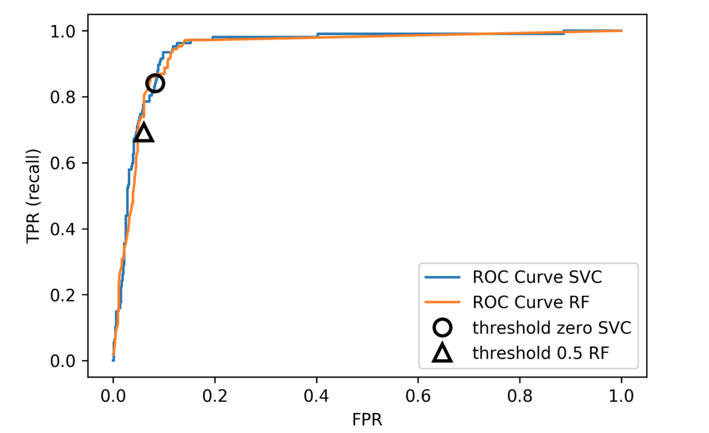
Roc Curve

.center[ ]

We also looked at ROC curves, which basically look at all possible thresholds as you can apply. Either for probabilistic prediction, or for any sort of continuous uncertainty estimate.

Remedies for the model

Today, I really want to talk about more, how we can change the model more than just changing the threshold. So how can we change the building of the model so that it takes into account the asymmetric costs, or asymmetric data.

Mammography Data

.smallest[ .left-column[

from sklearn.datasets import fetch_openml
## mammography https://www.openml.org/d/310
data = fetch_openml('mammography', as_frame=True)
X, y = data.data, data.target
X.shape

(11183, 6)

y.value_counts()

-1    10923
1       260

] .right-column[ .center[ ] ] .reset-column[

## make y boolean
## this allows sklearn to determine the positive class more easily
X_train, X_test, y_train, y_test = train_test_split(X, y == '1', random_state=0)

] ]

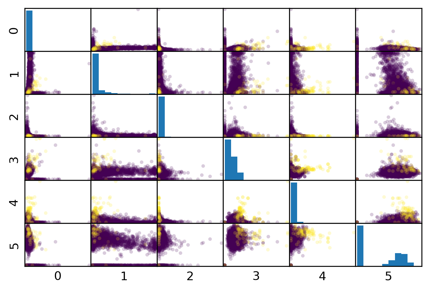
I use this mammography data set, which is very imbalanced. This is a data set that has many samples, only six features and it’s very imbalanced.

The datasets are about mammography data, and whether there are calcium deposits in the breast. They are often mistaken for cancer, which is why it’s good to detect them. Since its rigidly low dimensional, we can do a scatter plot. And we can see that these are much skewed distributions and there’s really a lot more of one class than the other.

Mammography Data

.smaller[

from sklearn.model_selection import cross_validate
from sklearn.linear_model import LogisticRegression

scores = cross_validate(LogisticRegression(),
                        X_train, y_train, cv=10,
                        scoring=('roc_auc', 'average_precision'))
scores['test_roc_auc'].mean(), scores['test_average_precision'].mean()

0.920, 0.630

from sklearn.ensemble import RandomForestClassifier
scores = cross_validate(RandomForestClassifier(),
                        X_train, y_train, cv=10,
                        scoring=('roc_auc', 'average_precision'))
scores['test_roc_auc'].mean(), scores['test_average_precision'].mean()

0.939, 0.722 ]

So as a baseline here is just evaluating logistic regression and the random forest on this. Actually, I ran it under ROC curve and average precision. I’ve used a cross-validate function model selection that allows you to specify multiple metrics. So I only need to train the model once but I can look at multiple metrics.

I do a 10 fold cross-validation on the data set and I split into training and test and so I can look at the scores here. The scores are dictionary, they give me training and test scores for all the metrics I specified. And so you can look at the mean test drug score and the mean test average precision score. This gives a high AUC and a quite low average precision.

Here is a second baseline with a random forest doing the same evaluation with ROC AUC and average precision. We get slightly higher AUC and quite a bit higher average precision.

Basic Approaches

.left-column[ .center[ ] ]

.right-column[

Change the training procedure ]

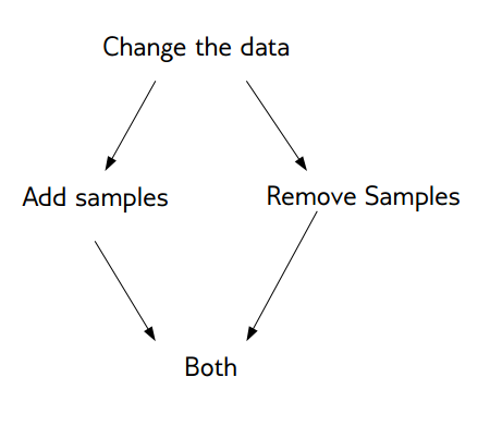
Now we want to change these basic training methods to be better adapted to this imbalanced dataset. There are generally two approaches. One is changing the data. And the other is change the training procedure and how you built the model. The easier one is to change the data. We can either add samples to the data, we can remove samples to the data, or we can do both. Resampling is not possible in scikit-learn because of some API issues.

Sckit-learn vs resampling

The problem with pipelines, as they’re in scikit-learn right now is, if you create a pipeline, and you call fit, it’ll always use the original y and the output of a transformer is always a transformed x. So we can’t change y. So we can re-sample the data.

• The transform method only transforms X

• Pipelines work by chaining transforms

• To resample the data, we need to also change y

Imbalance-Learn

http://imbalanced-learn.org

pip install -U imbalanced-learn

Extends sklearn API

So we’re going to use imbalance learn, which is an extension of the scikit-learn API that basically allows us to resample.

Sampler

To resample a data sets, each sampler implements:

  data_resampled, targets_resampled = obj.sample(data, targets)

Fitting and sampling can also be done in one step:

  data_resampled, targets_resampled = obj.fit_sample(data, targets)

–

In Pipelines: Sampling only done in fit!

This extends sampler objects in scikit-learn. The sampler objects have a sample method which returns resample data and resample targets.

There’s also pipelines in imbalance learn. The important part here is the sampling is only done in fit. So only your training data will be resampled. But when you do predictions, you want predictions to be made on the whole test set, and on the original test set. So you don’t want to mess with the test set in your evaluation. So resampling is only done when you’re building a model.

• Imbalance-learn extends scikit-learn interface with a “sample” method.

• Imbalance-learn has a custom pipeline that allows resampling.

• Imbalance-learn: resampling is only performed during fitting

• Warning: not everything in imbalance-learn is multiclass!

Random Undersampling

from imblearn.under_sampling import RandomUnderSampler
rus = RandomUnderSampler(replacement=False)
X_train_subsample, y_train_subsample = rus.fit_sample(
    X_train, y_train)
print(X_train.shape)
print(X_train_subsample.shape)
print(np.bincount(y_train_subsample))

(8387, 6)
(390, 6)
[195 195]

The easiest strategy is randomly undersampling. The default strategy is to undersample the majority class so that it has the same size as the minority class, that’s implemented in the random under sampler. Here, I instantiate to random under sampler, I set replacement equal to false, which means sampling without replacement and then I can do fit sample on the training set. And so the original training set was 8387 samples, the subsample data set is only 390 samples. And you can see now in the bin count here, the data set is balanced.

Basically, I reduced the majority class randomly to a very much smaller dataset, which made the majority class the same size as the minority class. And you can see that the dataset is 20 times smaller because the dataset was imbalanced. So building anything on this dataset will be much much faster. But also keep in mind, we threw away 98% of our data in doing that.

• Drop data from the majority class randomly

• Often untill balanced

• Very fast training (data shrinks to 2x minority)

• Loses data !

Random Undersampling

.smaller[

from imblearn.pipeline import make_pipeline as make_imb_pipeline

undersample_pipe = make_imb_pipeline(RandomUnderSampler(), LogisticRegressionCV())
scores = cross_validate(undersample_pipe,
                        X_train, y_train, cv=10,
                        scoring=('roc_auc', 'average_precision'))
scores['test_roc_auc'].mean(), scores['test_average_precision'].mean()
## baseline was 0.920, 0.630

0.927, 0.527

]

.smaller[

undersample_pipe_rf = make_imb_pipeline(RandomUnderSampler(),
                                        RandomForestClassifier())
scores = cross_validate(undersample_pipe_rf,
                        X_train, y_train, cv=10,
                        scoring=('roc_auc', 'average_precision'))
scores['test_roc_auc'].mean(), scores['test_average_precision'].mean()
## baseline was 0.939, 0.722

0.951, 0.629

]

Looking at the result, ROC AUC actually improved a little bit while the average precision decreased a little bit. Given that we threw away 98% of our data, I think the fact that the ROC AUC improved is quite remarkable. So this is clearly still a reasonable model, given one particular measure, it’s even a better model even though we threw away most of the data.

Even though it’s very simplistic, it’s actually a viable strategy that people often use in practice. In particular, if you have a very big data set, you might not have enough compute to actually do something on the whole dataset or you might only do something simple on the whole dataset. But after you resampled it, you can maybe train a much more complicated model.

Here by default, this random under simpler makes it balanced but of course, you could be slightly less extreme, so that you throw away a little bit fewer data.

We can do the same thing with random forest. After computing, the area under the ROC curve actually went up substantially. Again, it’s quite surprising given that we used much less data, but the average precision went down quite a bit.

• As accurate with fraction of samples!

• Really good for large datasets

Random Oversampling

from imblearn.over_sampling import RandomOverSampler
ros = RandomOverSampler()
X_train_oversample, y_train_oversample = ros.fit_sample(
    X_train, y_train)
print(X_train.shape)
print(X_train_oversample.shape)
print(np.bincount(y_train_oversample))

(8387, 6)
(16384, 6)
[8192 8192]

• Repeat samples from the minority class randomly

• Often untill balanced

• Much slower (dataset grows to 2x majority)

Random Oversampling

.smaller[

oversample_pipe = make_imb_pipeline(RandomOverSampler(), LogisticRegression())
scores = cross_validate(oversample_pipe,
                        X_train, y_train, cv=10,
                        scoring=('roc_auc', 'average_precision'))
scores['test_roc_auc'].mean(), scores['test_average_precision'].mean()
## baseline was 0.920, 0.630

0.917, 0.585 ]

.smaller[

oversample_pipe_rf = make_imb_pipeline(RandomOverSampler(),
                                       RandomForestClassifier())
scores = cross_validate(oversample_pipe_rf,
                        X_train, y_train, cv=10,
                        scoring=('roc_auc', 'average_precision'))
scores['test_roc_auc'].mean(), scores['test_average_precision'].mean()
## baseline was 0.939, 0.722

0.926, 0.715 ]

The complement of doing random sampling of the data is random oversampling of data. So in random oversampling, we do the opposite. We basically resample the training dataset so that the minority class has the same number of samples as the majority class.

Given that this dataset was very imbalanced, we nearly doubled the size of the training dataset. So now everything will be actually much slower because we have many more samples. We nearly doubled the dataset size because we reproduced many copies of the minority class and then we have a balanced dataset again.

Here, what we did is we just sampled with replacement. We sampled with replacement about 8000 times from this pool of 195 samples.

Q: Does that mean there are repeat records?

Yeah, most of them are repeated like 40 times on average.

Q: What distribution you’re sampling from?

We’re not sampling IID from the original distribution because in the original distribution there was a strongly imbalanced. So we now sample from the traditional distributions basically where we sample first the label and then we sample from this class. And we do this for the two labels independently in the same amount of time. It’s slightly weird because we have a lot of copies of the sample.

Logreg the same, Random Forest much worse than undersampling (about same as doing nothing)

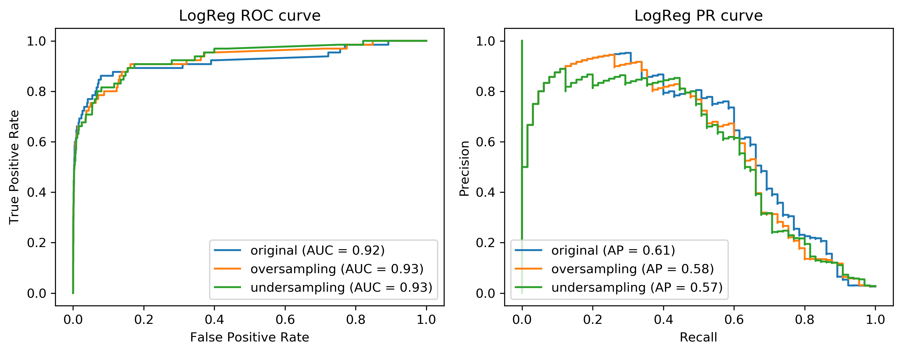
Curves for LogReg

.center[ ]

Here, I’m making a pipeline with logistic aggression random forest and you can see that the area under the ROC curve is actually lower, while the average precision is higher than with undersampling but slightly lower than the original dataset.

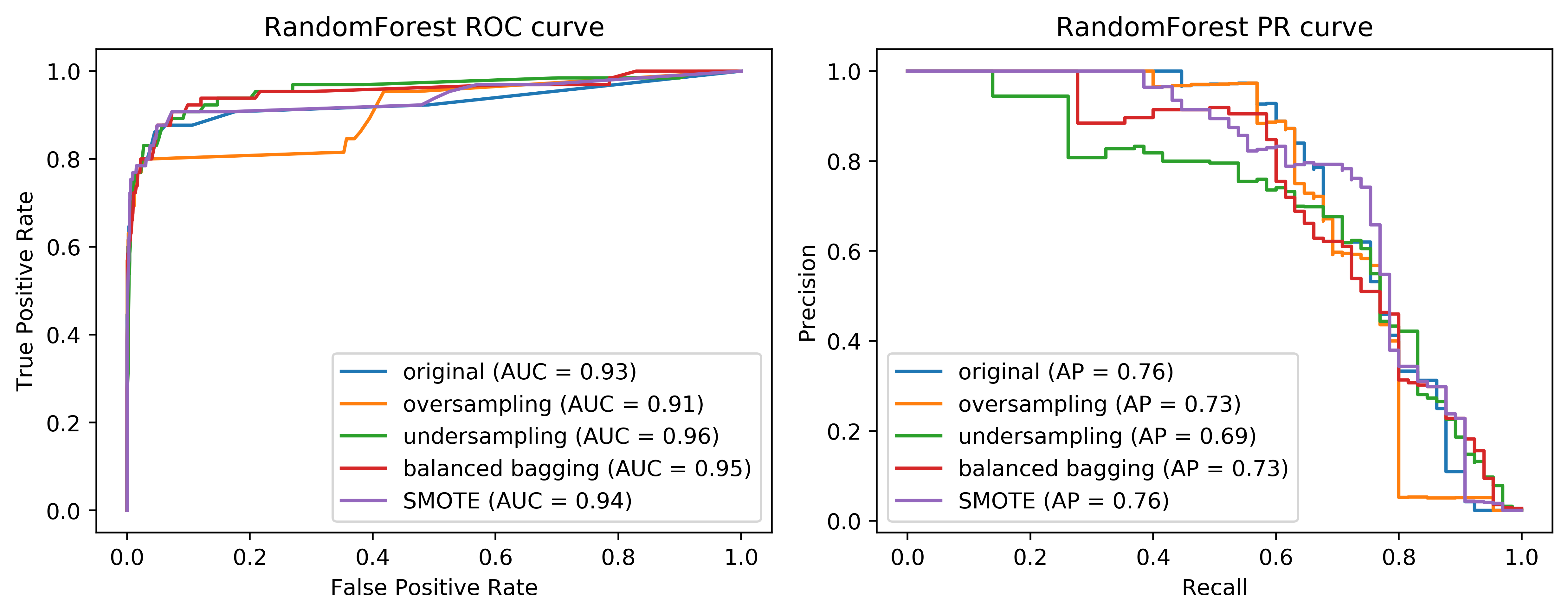
Curves for Random Forest

.center[ ]

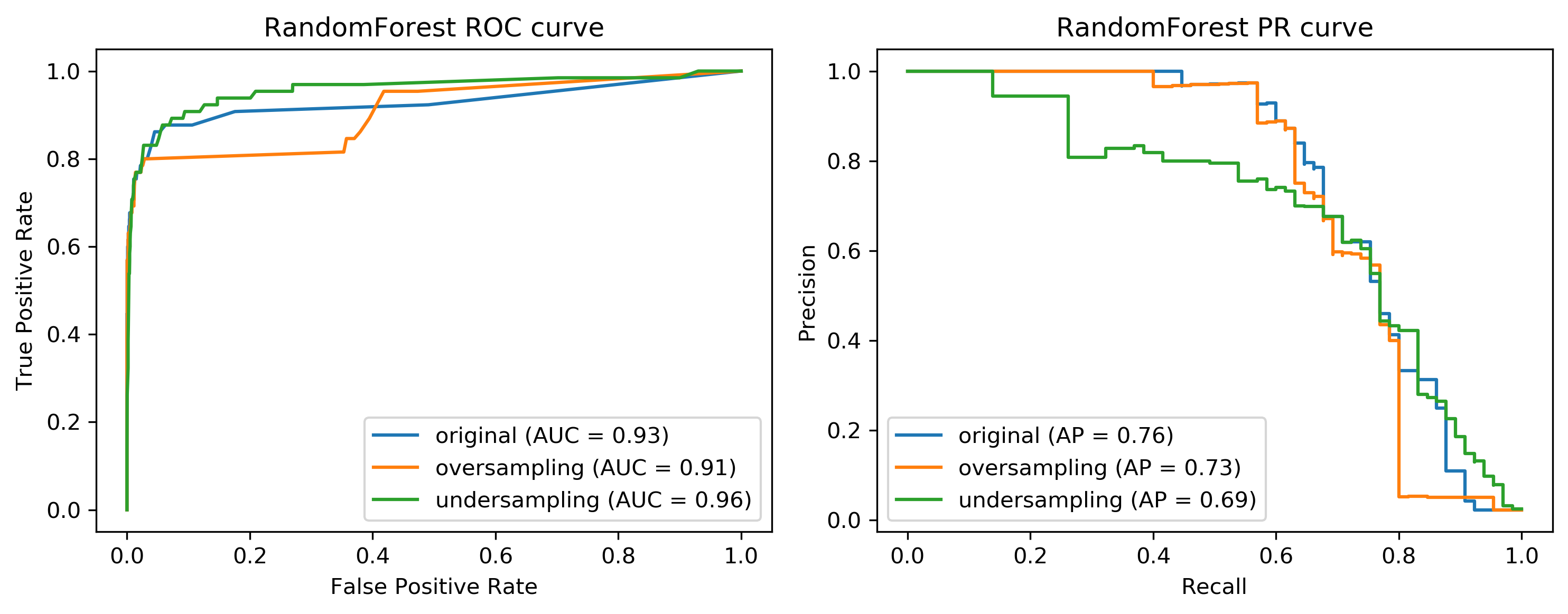We can also look at the curves. We have on the left, the ROC curve for logistic regression with the original data set, the oversample, and the under-sample dataset. On the right-hand side, we have the recall curve.

These are the same for random forest. If you look at these curves from afar, they give you the exact opposite ideas. On the left, under sample seems to be best and oversample is the worst while under sample is clearly the worst and under sample is not so bad on the curve in the right.

If I look at the precision-recall curve, the original data set did best. Looking at these two curves you get quite different ideas. The TPR axis is the same as the recall axis.

The idea is since we have the cost function, we know which could be the area under one of these curves, or could be a particular recall or position value or particular cost matrix we want to achieve and we want to optimize this. And we hope that by taking into account the imbalance of the classes, we can optimize this cost better than just basically using the IID data set. But precision and false positive rate measure quite different things.

Class-weights

• Instead of repeating samples, re-weight the loss function.

• Works for most models!

• Same effect as over-sampling (though not random), but not as expensive (dataset size the same).

One way we can make the resampling more efficient is by using class weights instead of actually resampling. So we can change our loss function to do the same thing as if you would resample but under sampling case, we don’t actually throw away any data and in the oversampling case, we don’t actually make our computational problem harder by repeating some of the samples. This works for most models and it’s pretty simple to do in scikit-learn. Basically, it’s the same as oversampling in a sense because you’re not throwing away any data.

Class-weights in linear models

\[\min_{w \in ℝ^{p}, b \in \mathbb{R}}-C \sum_{i=1}^n\log(\exp(-y_i(w^T \textbf{x}_i + b )) + 1) + ||w||_2^2\]

\[\min_{w \in ℝ^{p}, b \in \mathbb{R}}-C \sum_{i=1}^n c_{y_i} \log(\exp(-y_i(w^T \textbf{x}_i + b )) + 1) + ||w||_2^2\]

Similar for linear and non-linear SVM

So for the linear model, for example, let’s say we do logistic regression. Instead of minimizing this problem, for each class, we have a class weight c_(y_i ) and so the loss for each sample gets multiplied by this class weight and usually, they sum to one. This is similar to having a different penalty C for all of the different classes.

You can see that this is the same as if I repeat each sample x_i c_(y_i ) many times in each class. So if I set the cost weight of one class to 2, that would be the same as repeating each sample in this class twice, only now I don’t actually have to duplicate any sampling. So this is cheaper than over sampling but has the same effect.

You can do this for hinge loss and SVMs by just changing the loss.

Class weights in trees

Gini Index:

\[H_\text{gini}(X_m) = \sum_{k\in\mathcal{Y}} p_{mk} (1 - p_{mk})\]

\[H_\text{gini}(X_m) = \sum_{k\in\mathcal{Y}} c_k p_{mk} (1 - p_{mk})\]

Prediction:

Weighted vote

For trees and all trees based models, you can just change the splitting criteria. For example, if you have a Gini index here, and you compute the Gini index for each class or the cross-entropy for each class, and you have the class weights in here.

And again, you can see this is the same as replicating the data points c_k many times. If you want to make predictions, you can do a weighted vote.

#Using Class-Weights

.smaller[

scores = cross_validate(LogisticRegression(class_weight='balanced'),
                        X_train, y_train, cv=10,
                        scoring=('roc_auc', 'average_precision'))
scores['test_roc_auc'].mean(), scores['test_average_precision'].mean()
## baseline was 0.920, 0.630

0.918, 0.587

scores = cross_validate(RandomForestClassifier(n_estimators=100,
                                               class_weight='balanced'),
                        X_train, y_train, cv=10,
                        scoring=('roc_auc', 'average_precision'))
scores['test_roc_auc'].mean(), scores['test_average_precision'].mean()
## baseline was 0.939, 0.722

0.917, 0.701 ]

In scikit-learn, all the classifier has a class weight parameter. You can set them to anything you want, basically, giving arbitrary integers to the particular classes, there is normalized sum to one.

Balanced setting means do the same as oversampling so that the populations have the same size for all the classes. You can see this has a somewhat similar effect to the oversampling for only half the computational price.

This is a pretty simple way to try to change the model towards a positive class.

Ensemble Resampling

• Random resampling separate for each instance in an ensemble!

• Chen, Liaw, Breiman: “Using random forest to learn imbalanced data.”

• Paper: “Exploratory Undersampling for Class Imbalance Learning”

• Not in sklearn (yet)

• Easy with imblearn

There’s something a little bit better that’s called easy ensembles or resampling within an ensemble. So the idea is you build an ensemble like bagging classifier, but instead of doing a bootstrap sample, you can do a random undersampling into a balance dataset separately for each classifier in ensemble. Right now, you can only do this with imbalance learn.

Easy Ensemble with imblearn

.smaller[

from sklearn.tree import DecisionTreeClassifier
from imblearn.ensemble import BalancedBaggingClassifier

## from imblearn.ensemble import BalancedRandomForestClassifier
## resampled_rf = BalancedRandomForestClassifier()

tree = DecisionTreeClassifier(max_features='auto')
resampled_rf = BalancedBaggingClassifier(base_estimator=tree,
                                         random_state=0)
scores = cross_validate(resampled_rf,
                        X_train, y_train, cv=10,
                        scoring=('roc_auc', 'average_precision'))
scores['test_roc_auc'].mean(), scores['test_average_precision'].mean()
## baseline was 0.939, 0.722

0.957, 0.654

]

For example, I can do a balanced random forest, I’m using a decision tree as a base classifier with max features as auto. For classifier, this is the square root of number of features.

And so this will build 100 estimators. Each estimator will be basically trained on the random undersample of the data set. So I do a random under a sample of the data set 100 times and I build a tree on each of them. So this is exactly as expensive as building a random forest on the undersample data set, which is pretty cheap because under sampling throws away most of the data. In fact, we’re not throwing away as much data, we’re keeping a lot of the data but only in different trees in the ensemble.

Of all the models that we looked at today, this is the best one in terms of area under the curve. It’s cheap to do and it allows you to use a lot of your data in a pretty nice way. This has been shown to be like pretty competitive in a bunch of benchmarks.

-As cheap as undersampling, but much better results than anything else!

-Didn’t do anything for Logistic Regression.

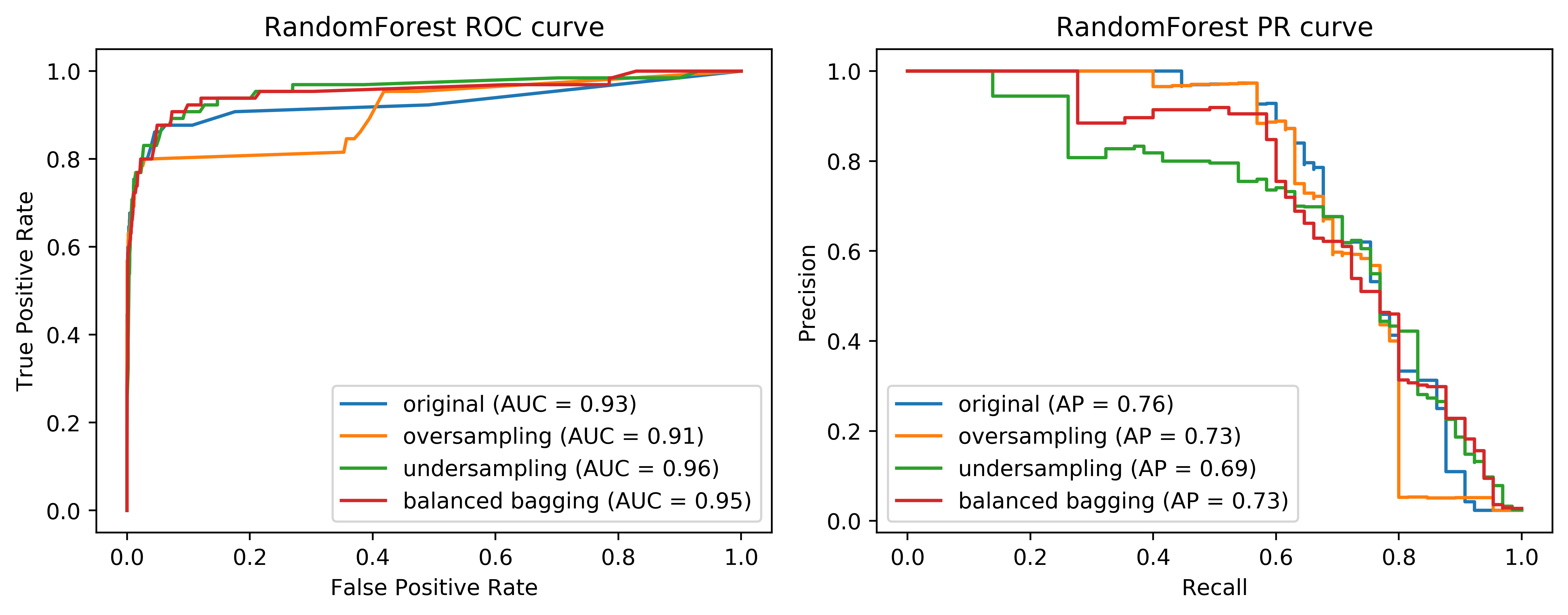
Looking at the curves again, comparing the easy ensemble. You can see that in the higher recall area, it does quite well and in the high precision area, it does better than just undersampling. So remember, this is much much cheaper than the oversampling by a large amount. And so if we are anywhere in this area here, it seems to be like a pretty decent solution.

To explain the difference between easy ensemble and under sample….In undersampling, I randomly under sample the dataset once. So then I have a balance dataset 195-195 and I built a model on this. And in this case, I build a random forest model. And in the easy ensemble, what I do is for each tree in the random forest I separately do an undersampling in 295-95. So they will all have the same minority class samples, but they all will have different majority class samples. So in total, I’m looking at more than 195 samples from the majority class since I under sample for each tree in a different way. That makes it quite a bit better.

These are all the randomly sample methods that I want to talk about. You can see that here, they make quite a big difference. Depending on where you want to be on this precision-recall curve, you would choose quite different methods.

Synthetic Sample Generation

There are many methods, but the only method that your interviewer will expect you to know is SMOTE.

Synthetic Minority Oversampling Technique (SMOTE)

• Adds synthetic interpolated data to smaller class

• For each sample in minority class:

  – Pick random neighbor from k neighbors.

  – Pick point on line connecting the two uniformly (or within rectangle)

  – Repeat.

I don’t think it’s actually used commonly in practice like the random oversampling and random undersampling. In particular, the undersample is great because it makes everything much faster.

The idea is to add samples to the smaller class. So you synthetically want to add samples that kind of looks like the smaller class and this way hopefully, bias the classifier more towards the smaller class. It’s also neighbor space so again if you have a very big dataset or if you’re in a very high dimension this might be slow. So in very high dimensions not even work that well.

So what we’re doing here is for each sample on the minority class you pick a random neighbor among the K nearest neighbors and then you pick a point on the line between the two.

• Leads to very large datasets (oversampling)

• Can be combined with undersampling strategies

.center[ ]

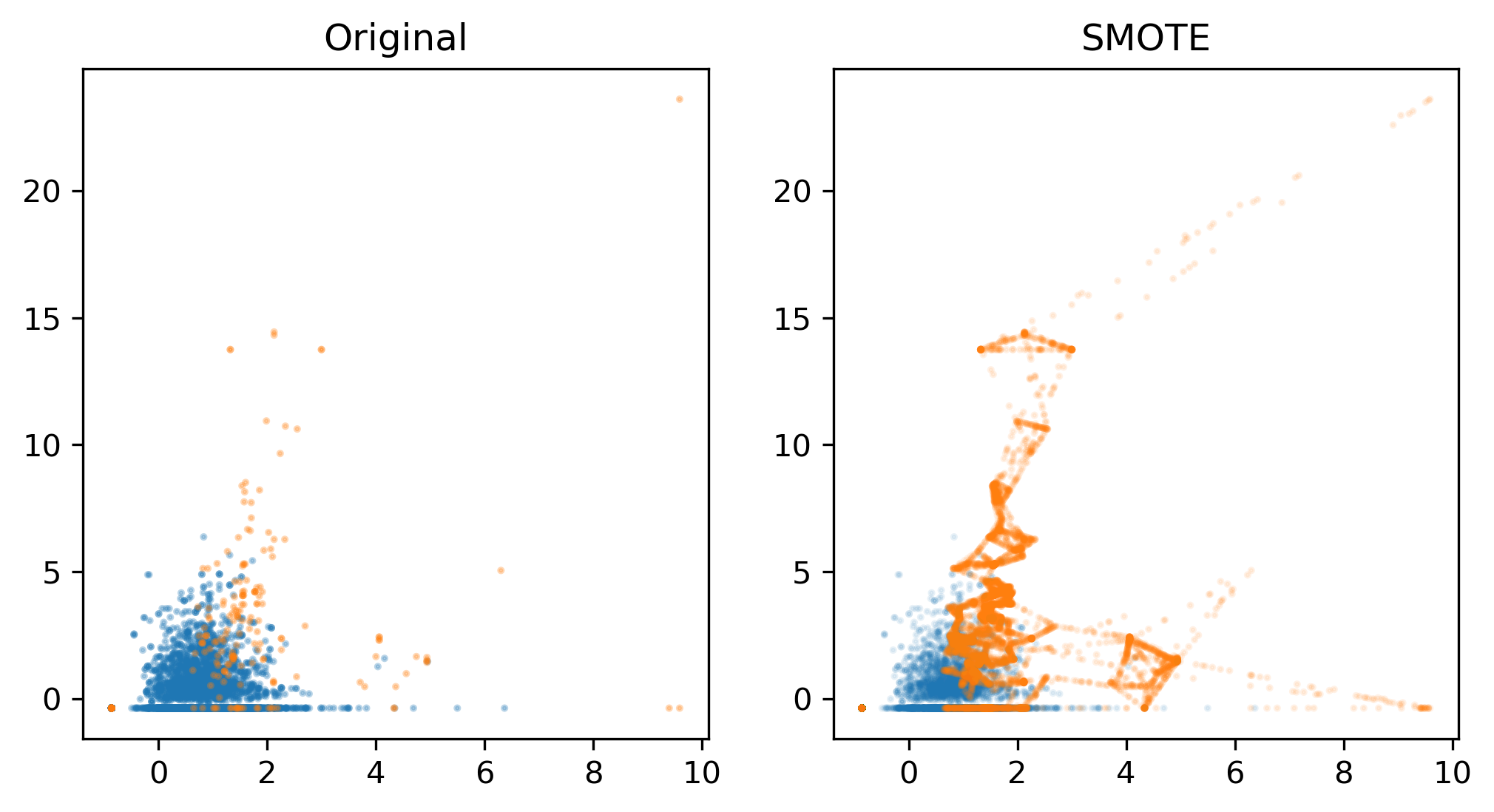This is feature three and feature four from the mammography dataset. You can see basically that for this dataset it’s pretty far away, K is three and so these neighbors were picked and then a bunch of times points was randomly picked on the line between the two. So basically, you get something that is sort of connecting all two data points.

This might set of make more sense than just repeating the sample over and over again. But also, if you’re in high dimensions, it’s not entirely clear how well this will work.

.smaller[

smote_pipe = make_imb_pipeline(SMOTE(), LogisticRegression())
scores = cross_validate(smote_pipe, X_train, y_train, cv=10,
                        scoring=('roc_auc', 'average_precision'))
pd.DataFrame(scores)[['test_roc_auc', 'test_average_precision']].mean()
## baseline was 0.920, 0.630

0.919, 0.585

smote_pipe_rf = make_imb_pipeline(SMOTE(),
                                  RandomForestClassifier())
scores = cross_validate(smote_pipe_rf, X_train, y_train, cv=10,
                        scoring=('roc_auc', 'average_precision'))
pd.DataFrame(scores)[['test_roc_auc', 'test_average_precision']].mean()
## baseline was 0.939, 0.722

0.946, 0.688

]

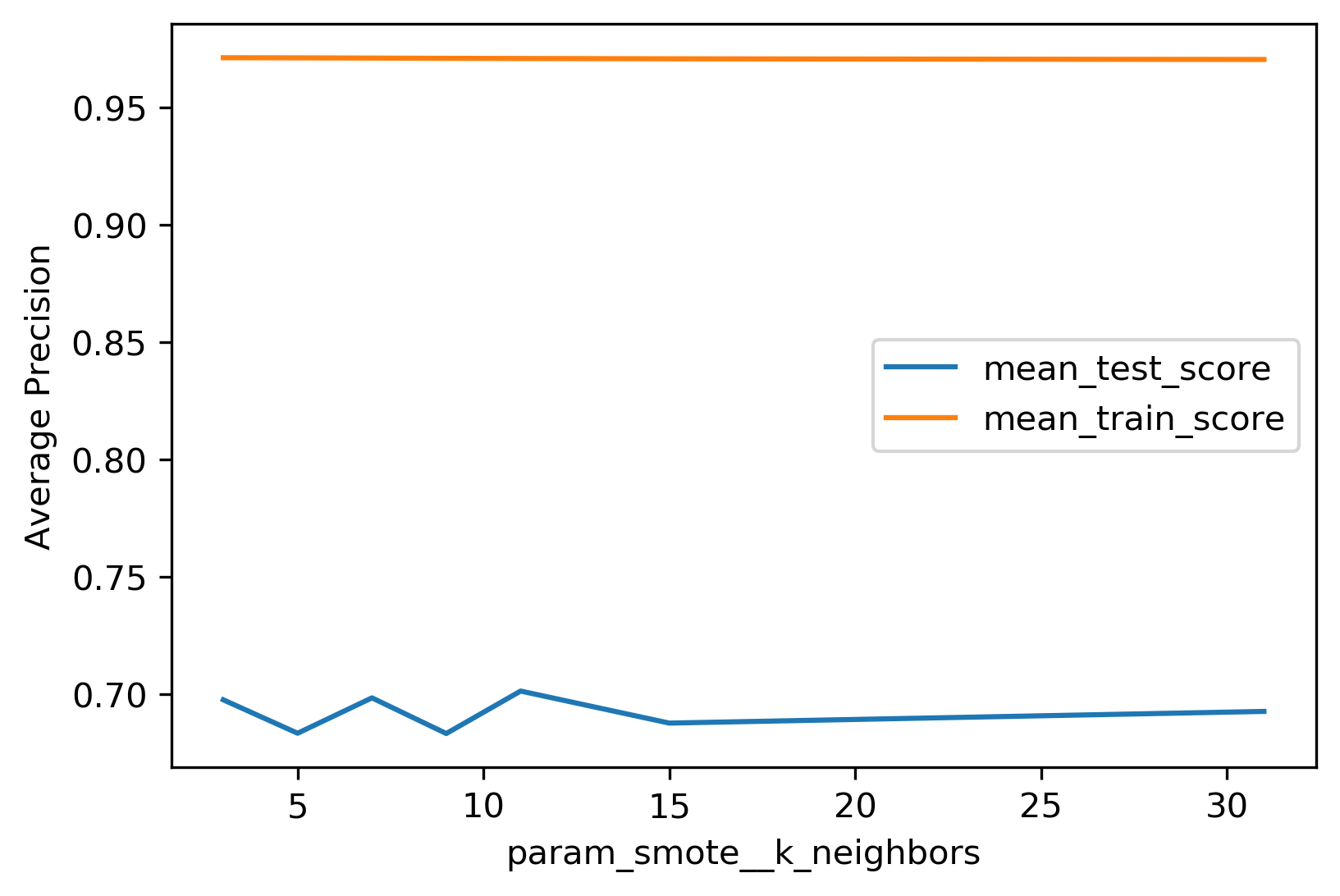
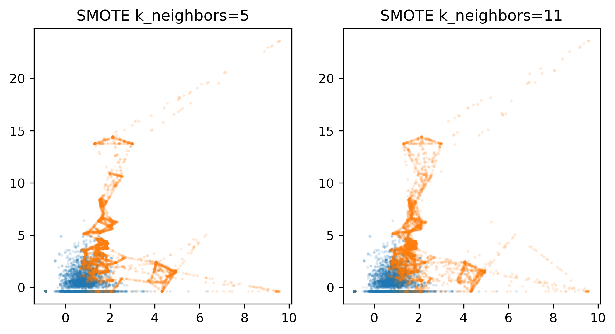
The results are pretty similar to either the original dataset or the random sampling. Performing nearest neighbors, I found 11 to be best.

.smaller[

param_grid = {'smote__k_neighbors': [3, 5, 7, 9, 11, 15, 31]}
search = GridSearchCV(smote_pipe_rf, param_grid, cv=10,
                      scoring="average_precision")
search.fit(X_train, y_train)
results = pd.DataFrame(search.cv_results_)
results.plot("param_smote__k_neighbors", ["mean_test_score", "mean_train_score"])

] .center[ ]

Also here in these plots, it looks now, there are more yellow points than purple points that’s because I followed the purple points first and then the yellow points. Because if I didn’t, then in the original data, you wouldn’t see any yellow points.

Again, if you look at the metrics, this doesn’t really make a big difference.

.center[ ]

.center[ ]

Summary

• Always check roc_auc and average_precision look at curves

• Undersampling is very fast and can help!

• Undersampling + Ensembles is very powerful!

• Can add synthetic samples with SMOTE

Always check the ROC AUC and the average precision and look at the curves. You’ve seen that the different strategies and different parts of the curves, they behave quite differently. Undersampling is really fast, and it can sometimes make things better. So I would always try under sampling just because maybe your model is slightly worse but if you get 100 times to speed up, it’s still worth it.

Using undersampling with easy ensembles is as fast as undersampling, but often gives better results.

People in machine learning research like balance datasets, but in the real world data sets are never balanced. Unfortunately, most of the datasets we have come from machine learning researchers. And so there’s really not a lot of interesting data sets that are very balanced.

The other thing I could have covered is you can directly optimize particular metrics. So you can train a model to optimize precision at K or area under the curve or something like that, at least for linear model, that’s relatively straightforward. I’m not sure what the outcome was if someone tried it with trees. But I think the most common is just reweighting to samples.

import numpy as np
import matplotlib.pyplot as plt
%matplotlib inline
np.set_printoptions(precision=3, suppress=True)
import pandas as pd
import sklearn
sklearn.set_config(print_changed_only=True)
from sklearn.model_selection import train_test_split, cross_val_score
from sklearn.pipeline import make_pipeline
from sklearn.preprocessing import scale, StandardScaler
import warnings
warnings.filterwarnings('ignore', category=DeprecationWarning)
warnings.filterwarnings('ignore', category=FutureWarning)

# mammography dataset https://www.openml.org/d/310
data = pd.read_csv("data/mammography.csv")

target = data['class']

target.value_counts()

y = (target != "'-1'").astype(np.int)
y.value_counts()

X = data.iloc[:, :-1]
X.shape

X.hist(bins='auto')

pd.plotting.scatter_matrix(X, c=y, alpha=.2);

X_train, X_test, y_train, y_test = train_test_split(
    X.values, y.values, stratify=y, random_state=0)

from sklearn.model_selection import cross_validate
from sklearn.linear_model import LogisticRegression

scores = cross_validate(LogisticRegression(),
                        X_train, y_train, cv=10, scoring=('roc_auc', 'average_precision'))
scores['test_roc_auc'].mean(), scores['test_average_precision'].mean()

from sklearn.ensemble import RandomForestClassifier
scores = cross_validate(RandomForestClassifier(n_estimators=100),
                        X_train, y_train, cv=10, scoring=('roc_auc', 'average_precision'))
scores['test_roc_auc'].mean(), scores['test_average_precision'].mean()

from imblearn.under_sampling import RandomUnderSampler

rus = RandomUnderSampler(replacement=False)
X_train_subsample, y_train_subsample = rus.fit_sample(X_train, y_train)
print(X_train.shape)
print(X_train_subsample.shape)
print(np.bincount(y_train_subsample))

from imblearn.pipeline import make_pipeline as make_imb_pipeline

undersample_pipe = make_imb_pipeline(RandomUnderSampler(), LogisticRegression())
scores = cross_validate(undersample_pipe,
                        X_train, y_train, cv=10, scoring=('roc_auc', 'average_precision'))
scores['test_roc_auc'].mean(), scores['test_average_precision'].mean()

from imblearn.over_sampling import RandomOverSampler
ros = RandomOverSampler()
X_train_oversample, y_train_oversample = ros.fit_sample(X_train, y_train)
print(X_train.shape)
print(X_train_oversample.shape)
print(np.bincount(y_train_oversample))

oversample_pipe = make_imb_pipeline(RandomOverSampler(), LogisticRegression())
scores = cross_validate(oversample_pipe,
                        X_train, y_train, cv=10, scoring=('roc_auc', 'average_precision'))
scores['test_roc_auc'].mean(), scores['test_average_precision'].mean()

undersample_pipe_rf = make_imb_pipeline(RandomUnderSampler(), RandomForestClassifier(n_estimators=100))
scores = cross_validate(undersample_pipe_rf,
                        X_train, y_train, cv=10, scoring=('roc_auc', 'average_precision'))
scores['test_roc_auc'].mean(), scores['test_average_precision'].mean()

oversample_pipe_rf = make_imb_pipeline(RandomOverSampler(), RandomForestClassifier(n_estimators=100))
scores = cross_validate(oversample_pipe_rf,
                        X_train, y_train, cv=10, scoring=('roc_auc', 'average_precision'))
scores['test_roc_auc'].mean(), scores['test_average_precision'].mean()

Class Weights

scores = cross_validate(LogisticRegression(class_weight='balanced'),
                        X_train, y_train, cv=10, scoring=('roc_auc', 'average_precision'))
scores['test_roc_auc'].mean(), scores['test_average_precision'].mean()

scores = cross_validate(RandomForestClassifier(n_estimators=100, class_weight='balanced'),
                        X_train, y_train, cv=10, scoring=('roc_auc', 'average_precision'))
scores['test_roc_auc'].mean(), scores['test_average_precision'].mean()

Resampled Ensembles

from sklearn.tree import DecisionTreeClassifier
from imblearn.ensemble import BalancedRandomForestClassifier
resampled_rf = BalancedRandomForestClassifier(n_estimators=100, random_state=0)

scores = cross_validate(resampled_rf,
                        X_train, y_train, cv=10, scoring=('roc_auc', 'average_precision'))
scores['test_roc_auc'].mean(), scores['test_average_precision'].mean()

GridSearchCV(scoring=('roc_auc', 'average_precision'), refit='average_precision')

GridSearchCV(scoring=('roc_auc', 'average_precision'), refit=False)

Exercise

Pick two or three of the models and strategies above, run grid-search (optimizing roc_auc or average precision), and plot the roc curves and PR-curves for these models.

Feature Engineering Automatic Feature Selection