import numpy as np
import matplotlib.pyplot as plt
import pandas as pd
%matplotlib inline
import sklearn
sklearn.set_config(print_changed_only=True)
Automatic Feature Selection
Univariate statistics
Feature Selection
Alright, so let’s talk about automatic feature selection. I want to talk about what methods are there to determine what features are important for your dataset, what features are important for a particular model.
Why Select Features?
Avoid overfitting (?)
Faster prediction and training
Less storage for model and dataset
More interpretable model
There’s a couple of reasons why you might want to feature selection. One is to avoid overfitting and get a better model. In practice, I have rarely seen that happen. It’s not usually what I would try to do to increase performance. If I’m only interested in performance I probably would not try to do automatic feature selection unless I think only a very small subset of my feature is actually important. There’s a lot of increasing performance just by selecting only important features.
What I think is more commonly, the reason to do automatic feature selection is you want to shrink your model to make faster predictions, to train your model faster, to store fewer data and possibly to collect fewer data. If you’re collecting the data or to feature from some online process, maybe it means you need fewer features, you need to store less information. I think actually the top reason to do feature selection is to have a more interpretable model. If your model is smaller, if your model has 5 features instead of 500, it’s probably much easier for you to grasp what the model does. If you can have a model that is as good with way fewer features, it will be much easier to explain and most people will be happy with it.
Types of Feature Selection
Unsupervised vs Supervised
Univariate vs Multivariate
Model based or not
There’s a couple of different types of feature selection that I want to talk about. You can have supervised and unsupervised feature selection. Depending on whether you consider the target or not. You can have Univariate versus Multivariate feature selection. Whereas Univariate looks at each feature at a time and determines if it’s important. Multivariate looks at interactions as well. And you can have a feature selection based on a particular machine learning model or not.
Unsupervised Feature Selection
May discard important information
Variance-based: 0 variance or mostly constant
Covariance-based: remove correlated features
PCA: remove linear subspaces
So the simpler thing that you might try is to do unsupervised feature selection which means just discard some features based on the statistics. For example, you could remove features that are mostly constant or that have zero variance. Like if they’re always constant, then definitely they’re not going to help you and you can remove them. If they have very small variance, on the other hand, that might only mean the scale of the features is small and you should just re-scale the feature. So just because it has a small variance, it doesn’t really mean anything. People often discard covariance features. But maybe just the difference between these two correlated features was the thing that’s important for prediction. If you use any unsupervised method, then you don’t know what are the things that are actually important are. Similarly, with PCA, it’s not really feature selection, because it doesn’t select subsets of the original feature. PCA will always use all original features. But it will remove linear subspaces of the feature space. And again, a lot of people like this to reduce the dimensionality and you will get the same things like a smaller model, maybe not more interpretable. It might be that the information you discarded is just the information that’s important. In a covariance sense, just because the data doesn’t extend a lot in a particular direction doesn’t mean that this direction isn’t the most important one for your prediction problem.
Covariance
.smaller[
from sklearn.preprocessing import scale

boston = load_boston()
X, y = boston.data, boston.target
X_train, X_test, y_train, y_test = train_test_split(X, y, random_state=0)
X_train_scaled = scale(X_train)

cov = np.cov(X_train_scaled, rowvar=False)
]
.center[
 ]
]
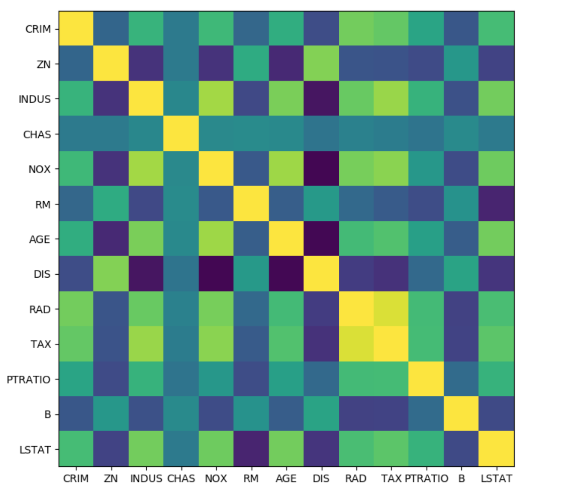
Here’s what the covariance matrix looks like for the Boston housing data set. The way you could do covariance based feature selection is you look at the features that have the highest covariance and just drop one of them or you could sum over all the features and look at which features most correlated with the other ones and drop that.
from scipy.cluster import hierarchy
order = np.array(hierarchy.dendrogram(
    hierarchy.ward(cov),no_plot=True)['ivl'], dtype="int")
.center[
 ]
]
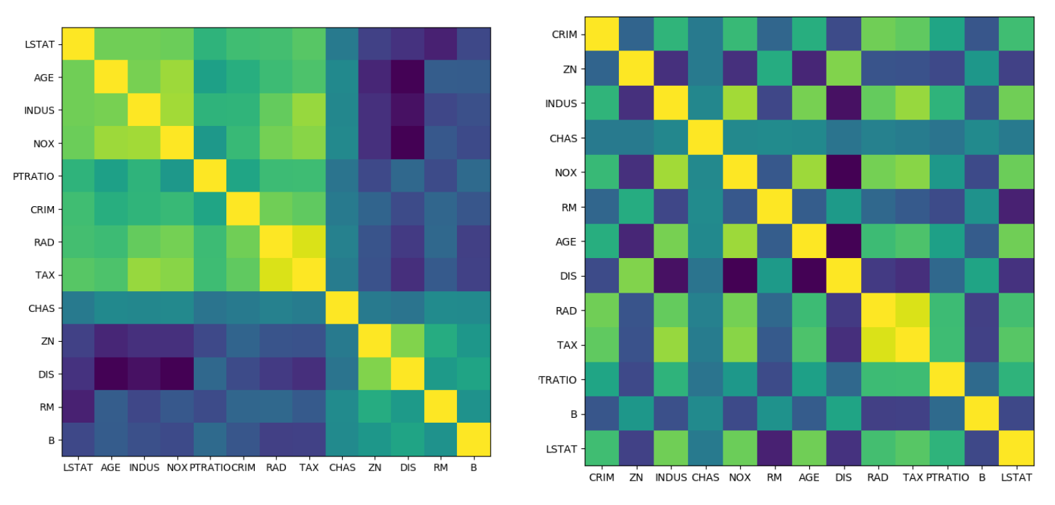
So if you look at covariance, it should probably try to sort your features using some clustering. Here I’m using hierarchical clustering from scipy. On the right, it’s the covariance matrix and on the left, it’s also the covariance matrix where I reordered the columns and rows. You can see that there are three correlated blocks. You could do this automatically, or you could look at it and see what you think how many features are there, and how many of them are correlated. I really urge you, whenever you look at correlation, never look at correlation without resorting the columns. On the right-hand side here, maybe I can see that these two are correlated, but I can’t see anything else. Whereas on the left hand I can see much more clearly what the structure of the data is. What it did just was, it did clustering on the rows and columns to resort them.
Supervised Feature Selection
Univariate Statistics
.smaller[
Pick statistic, check p-values !
f_regression, f_classsif, chi2 in scikit-learn
from sklearn.feature_selection import f_regression
f_values, p_values = f_regression(X, y)
]
.center[
 ]
]
So the simplest way is univariate features selection without models. The most classical one is to use statistical test and see the ones that are significantly related to the target. Depending on whether you look through classification or regression, you can add a t-test, f-test or chi-squared test and you can say which are the features that are significantly related with a target and I’m just going to select these.
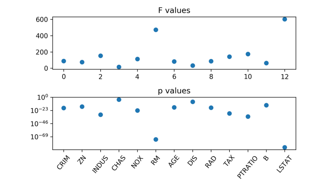
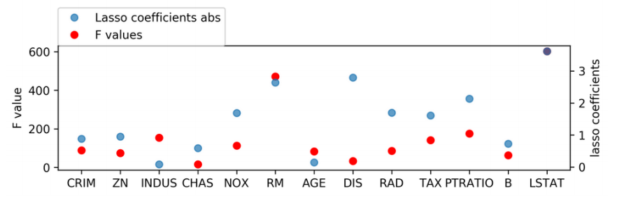
So this is again here for the Boston housing dataset, using F regression and F test. You can see here F values and the P values and you could use either of them to select a subset of the features. So for example, the number of rooms and LSTAT had very high F values, very small P values. These are certainly the most important features. While this one here doesn’t seem very important. One reason why this is not very important is because this is the binary variable and so this assumes linear regression model and the linear regression model is not very good at exploiting the binary variable.
This is a super quick test to do. It’s very fast, it’s probably something you want to look at. But it assumes a linear model, which you might not want to assume.
.smaller[
from sklearn.feature_selection import SelectKBest, SelectPercentile, SelectFpr
from sklearn.linear_model import RidgeCV

select = SelectKBest(k=2, score_func=f_regression)
select.fit(X_train, y_train)
print(X_train.shape)
print(select.transform(X_train).shape)
(379, 13)
(379, 2)
]
.smaller[
all_features = make_pipeline(StandardScaler(), RidgeCV())
np.mean(cross_val_score(all_features, X_train, y_train, cv=10))
0.718 ]
.smaller[
select_2 = make_pipeline(StandardScaler(),
                         SelectKBest(k=2, score_func=f_regression), RidgeCV())
np.mean(cross_val_score(select_2, X_train, y_train, cv=10))
0.624 ]
If you want to use these univariate statistics in scikit-learn there’s a couple of tools to select features based on this. In feature selection, there’s a whole bunch of them. There select k best which selects the K best feature, you can specify the number of features you want. Select percentile, which selects a percentile that you want and then there’s select FPR, it controls for the false positive rate, it basically does the multiple hypothesis testing adjustments to make sure that you false discovery rate of thinking the features are significantly important is low. These are scikit-learn transformers, you can instantiate them. By default, the parameter they all use a score function for classification. So if you want to do regression, you need to set the score function to F regression because you need different tests for regression classification. I said linear regression is not for binary features, maybe I shouldn’t have formulated in that way. Linear regression doesn’t allow you to do interactions, which is if you have multiple binary features would be the only issue. It’s more sort of that this linear test will not put a lot of emphasis on a binary feature because the way the test works. I can obviously also put this in a pipeline. Here, I’ve used a centered scale for ridge in a pipeline for a Boston housing data set and here, I’ve used two best features. You can see it actually got much worse because two features are not enough to select or to express all the information.
Mututal Information
from sklearn.feature_selection import mutual_info_regression
scores = mutual_info_regression(X_train, y_train,
                                discrete_features=[3])
.center[
 ]
]
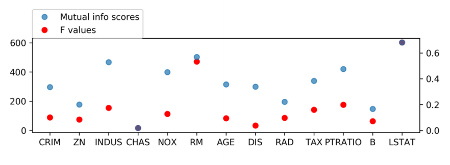
Another univariate statistics that you can use which is a little bit more complicated, which is called Mutual Information. There’s a version for regression classification in scikit-learn. This doesn’t use a linear model. It uses a non-parametric model using nearest neighbors. So basically, this also works if the interaction is nonlinear and it works on discrete and continuous features, but you have to tell us which features are discrete. So here, in this case, I tell it the feature number three is discrete and then this gives me some scores telling me what’s the mutual information between this feature in the target. Here I’m comparing the F values off the standard regression tests with the mutual information and they are sort of similar, but not entirely. If you think there are nonlinear interactions, and you have a model that can capture nonlinear interactions, then doing feature selection like taking these nonlinear features into account is good. This is much more computationally intensive than doing the F statistics. But this is still Univariate, looking at one feature at a time.
#Model-Based Feature Selection
Get best fit for a particular model
Ideally: exhaustive search over all possible combinations
Exhaustive is infeasible (and has multiple testing issues)
Use heuristics in practice.
So now let’s look at multiple features at a time. Most of the things that look at multiple features at a time are model-based. Usually, model-based feature selection finds the subset of features on which this model performs best. So giving them a particular model like a linear model, or random forest, I want to find a subset of features for which this model performs best in terms of cross-validation performance. Ideally, to do that, I would do an exhaustive search over all possible subsets of the features. But that’s like exponentially many. Also, if I do so many models fits I might overfit. So instead, there are several heuristics you can use to basically shrink or grow the sets of features that you’re using.
So first you fix the model. For models that give you some measure of feature importance, there’s a very simple technique which just looks at how important the models feature is.
Model based (single fit)
.smaller[
Build a model, select “features important to model”
Lasso, other linear models, tree-based Models
Multivariate - linear models assume linear relation ] .smaller[
from sklearn.linear_model import LassoCV
X_train_scaled = scale(X_train)
lasso = LassoCV().fit(X_train_scaled, y_train)
print(lasso.coef_)
[-0.881 0.951 -0.082 0.59 -1.69 2.639 -0.146 -2.796 1.695 -1.614 -2.133 0.729 -3.615] ]
.center[
 ]
]
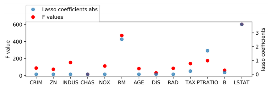
Using, say, a linear model, you fit the single model, and you discard all the features that the model doesn’t think are important. So this works for linear models really well and for tree-based models. This allows you to take linear interactions into account and with trees it allows you to take arbitrary interactions into account. So for example, I can use lasso, I can fit the lasso on my model, and I can look at the coefficients and the things that have small coefficients are less important in some sense, and so I could discard some of them. Here again, I plot the F values versus the coefficients of lasso. For example, here you can see for this variable, Lasso thinks its way less important than Univariate selection. Maybe because it was explained already by a combination of the other features. So if you have very co-related features Univariate selection will give all of them the same importance whereas lasso will usually pick only one of them. If you have many co-related features lasso picks only one of them at random. So it doesn’t mean that other features are not important. Question is what does this purple don’t represent? It represents that both the points are overlapping entirely.
Here I use lassoCV which means it adjusted the regularization parameter in Lasso to make the optimum predictions.
Changing Lasso alpha
.smaller[
from sklearn.linear_model import Lasso
X_train_scaled = scale(X_train)
lasso = Lasso().fit(X_train_scaled, y_train)
print(lasso.coef_)
[-0. 0. -0. 0. -0. 2.529 -0. -0. -0. -0.228 -1.701 0.132 -3.606] ]
.center[
 ]
]
If I look at the different alpha, it might be quite different. For example here with a default alpha of one, a lot of the coefficients are exactly zero and you can see it would only select five. How to select the alpha in lasso is important for the feature selection and so you might want to grid search. Now, let’s say we want to use this and so we want a scikit-learn estimator that does this. So we can put it in a pipeline.
SelectFromModel
from sklearn.feature_selection import SelectFromModel
select_lassocv = SelectFromModel(LassoCV(), threshold=1e-5)
select_lassocv.fit(X_train, y_train)
print(select_lassocv.transform(X_train).shape)
(379,11)
–
pipe_lassocv = make_pipeline(StandardScaler(), select_lassocv, RidgeCV())
np.mean(cross_val_score(pipe_lassocv, X_train, y_train, cv=10))
np.mean(cross_val_score(all_features, X_train, y_train, cv=10))
0.717
0.718
–
## could grid-search alpha in lasso
select_lasso = SelectFromModel(Lasso())
pipe_lasso = make_pipeline(StandardScaler(), select_lasso, RidgeCV())
np.mean(cross_val_score(pipe_lasso, X_train, y_train, cv=10))
0.671
SelectFrom model will work with any model with coef_ or feature_importances_. So that’s any linear model or tree based model. It uses this to select the features. So this will fit lasso and then if you call transform, it will discard all the features that lasso thought are not important. And you can change the threshold here, for example, so in this case, here I want to discard everything that lasso put to zero so I put a very small threshold in there. I could also set the threshold to be the median which selects 50% of the features. Here we are possibly discarding multiple features at once. SelectFromModel fits a single model, gets the feature importance was from this model and then drops according to the feature importance. And so here is how it looks in the pipeline, for example, you can see here that lasso with these parameters, drop two of the features and 11 after 13 remains. If I put it in a pipeline the performance is about the same.
Iterative Model-Based Selection
Fit model, find least important feature, remove, iterate.
Or: Start with single feature, find most important feature, add, iterate.
But maybe dropping multiple features at once is not a good idea because the importance of the features might change once we dropped some of them. What we can do is, we can iteratively build models. And we could either start with a single feature then add more important ones or we could start with all features and discard some.
We’ll talk about these two strategies which are slightly different.
Recursive Feature Elimination
Uses feature importances / coefficients, similar to “SelectFromModel”
Iteratively removes features (one by one or in groups)
Runtime: (n_features - n_feature_to_keep) / stepsize
So the next step from what we just saw would be recursive feature elimination. So if we use SelectFromModel it will drop all the unimportant features at once, in a recursive feature elimination usually drops one feature at a time or as a parameter step size it drops step size features at a time. So you fit the model, you discard the least important feature, you fit the model, you discard the important feature and so on until you have as many features left as you want again. Again, this needs the model to meet some measure of feature importance so you can use this with the linear model or tree-based model. An example where you cannot use this is, at least not in scikit-learn is Kernel SVM or neural networks, because they don’t really give you a measure of feature importance easily. For each step feature that we remove, we need to train a new model. So this is much more expensive because we need to retrain the model many times, but we’re sort of being more careful in how we remove the features.
.smaller[
from sklearn.linear_model import LinearRegression
from sklearn.feature_selection import RFE

## create ranking among all features by selecting only one
rfe = RFE(LinearRegression(), n_features_to_select=1)
rfe.fit(X_train_scaled, y_train)
rfe.ranking_
array([ 9, 8, 13, 11, 5, 2, 12, 4, 7, 6, 3, 10, 1]) ]
.center[
 ]
]
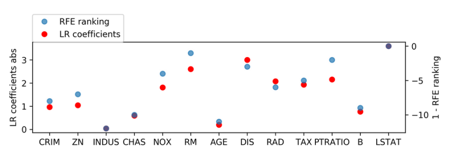
This is implemented in RFE, for recursive feature elimination, it works similar to SelectFromModel. To do RFE, then the model that you want to use and then you can specify how many features you want to select. Here I’m comparing the ranking according to RFE. So when it dropped out the features to the linear regression coefficients, which is basically what I would use if I drop them off all at once, and you can see that they’re sort of similar. So there’s probably not a whole lot of difference, at least in this case. You need to specify how many features you want to select. But if you want to select only one feature, you have to build many models and drop all the other features and so on the way you tried out the model for keeping five features and so on. So if you want a grid search this, doing this independently would be a whole waste of time because they would do the same thing over and over again.
RFECV
.smaller[
from sklearn.linear_model import LinearRegression
from sklearn.feature_selection import RFECV
rfe = RFECV(LinearRegression(), cv=10)
rfe.fit(X_train_scaled, y_train)
print(rfe.support_)
print(boston.feature_names[rfe.support_])
[ True  True False  True  True  True False  True  True  True  True  True
  True]
['CRIM' 'ZN' 'CHAS' 'NOX' 'RM' 'DIS' 'RAD' 'TAX' 'PTRATIO' 'B' 'LSTAT']
pipe_rfe_ridgecv = make_pipeline(StandardScaler(),
                                 RFECV(LinearRegression(), cv=10), RidgeCV())
np.mean(cross_val_score(pipe_rfe_ridgecv, X_train, y_train, cv=10))
0.710
]
So there’s a thing called RFECV that allows you to do efficient grid search for the number of features to keep. This basically has built-in cross-validation, provides the number of features to keep.
I’ve done RFECVC with linear regression and set it to do 10 fold cross-validation and then it will do the recursive feature elimination inside cross-validation and so it goes down from all features to just having one feature and with cross-validation, it will select the best number.
.smaller[
pipe_rfe_ridgecv = make_pipeline(StandardScaler(),
                                 RFECV(LinearRegression(), cv=10), RidgeCV())
np.mean(cross_val_score(pipe_rfe_ridgecv, X_train, y_train, cv=10))
0.710
from sklearn.preprocessing import PolynomialFeatures
pipe_rfe_ridgecv = make_pipeline(StandardScaler(), PolynomialFeatures(),
                                 RFECV(LinearRegression(), cv=10), RidgeCV())
np.mean(cross_val_score(pipe_rfe_ridgecv, X_train, y_train, cv=10))
0.820
]
If we want to predict with the same model as used for selection, RFECV can be used as the prediction step. Could also use RFECV as transformer and use any other model!
Wrapper Methods
Can be applied for ANY model!
Shrink / grow feature set by greedy search
Called Forward or Backward selection
Run CV / train-val split per feature
Complexity: n_features * (n_features + 1) / 2
Implemented in mlxtend
So as I set recourse to each elimination. So this is more careful and it requires the model that gives you feature importance. There’s sort of more general reprimand sets that are, in a sense, even more careful, but also more expensive, but it can be applied to any model. These are sequential feature selection. The idea is to either start with zero features, and add the most important feature, or start with all features and remove the least important feature at a time. And you do this by not using a feature importance by the model. But actually each step you basically do like one step looking at search. So let’s say I started with all the features, I leave out the first feature, build the model and but I don’t only build a model, I do cross-validation of the model on the subset so I get some accuracy or R squared value. And I do this for every single feature. So I leave each feature out and look at the cross-validate accuracy. And I dropped the one that gives me the highest cost-validated accuracy.
So now basically, this is even more expensive than doing the recursive feature elimination because I do a one step, look ahead. So now the runtime is quadratic in the number of features. Also for each iteration, I not only need to train a single model, I need to do cross-validation.
This is like a pretty standard method, because it’s like very general, and you can apply it to any model. It’s like a brute force search. Right now it’s not in scikit-learn, but it’s in a package called mlxtend which has a couple other tools.
Mlxtend is luckily fully scikit-learn compatible, so you can put it in a pipeline and everything’s fine.
SequentialFeatureSelector
.smaller[
from mlxtend.feature_selection import SequentialFeatureSelector
sfs = SequentialFeatureSelector(LinearRegression(), forward=False, k_features=7)
sfs.fit(X_train_scaled, y_train)
Features: 7/7
print(sfs.k_feature_idx_)
print(boston.feature_names[np.array(sfs.k_feature_idx_)])
(1, 4, 5, 7, 9, 10, 12)
['ZN' 'NOX' 'RM' 'DIS' 'TAX' 'PTRATIO' 'LSTAT']
sfs.k_score_
0.725
]
So from mlxtend, you get feature selection, sequential feature selector, you put into the model, you tell it whether you want to do forward or backward. Forward equal to false means I started with all and I prune features one by one. Forward equal to true means I start with zero features and I use the one that gives me highest accuracy and then I add one by one. As I said with sequential feature selector, you need to specify the number of features and it does internally cross-validation and it optimizes accuracy for classification models and r square for regression models and does this stepwise selection. One thing I should have mentioned if you do feature selection this way, theoretically, you can have a model for feature selection that’s different from the model for prediction. In here, if you look at the top for the recursive feature elimination, I use linear regression. But actually, the model I fit in the end was a ridge model. So I could also use, let’s say, a tree-based model for feature selection and then the linear model for prediction if I wanted to. It’s not entirely clear if that helps or makes sense, but it’s sort of an additional degree of freedom. And for example, if I want a very interpretable model, I want my model that does the predictions to be linear so I can explain to my boss what it means. But I can also still do the feature selection using a more complicated model and just tell my boss “Oh, only these features are important and here’s how I make the prediction”
Questions ?
The question is if I do forward method or backward method with the same number of features will the same happen? They both are sort of one step look ahead approximations to trying out all subsets and there’s no guarantee we would get the same thing.
from sklearn.datasets import load_breast_cancer
from sklearn.feature_selection import SelectPercentile
from sklearn.model_selection import train_test_split

cancer = load_breast_cancer()

# get deterministic random numbers
rng = np.random.RandomState(42)
noise = rng.normal(size=(len(cancer.data), 50))
# add noise features to the data
# the first 30 features are from the dataset, the next 50 are noise
X_w_noise = np.hstack([cancer.data, noise])

X_train, X_test, y_train, y_test = train_test_split(
    X_w_noise, cancer.target, random_state=0, test_size=.5)
# use f_classif (the default) and SelectPercentile to select 10% of features:
select = SelectPercentile(percentile=50)
select.fit(X_train, y_train)
# transform training set:
X_train_selected = select.transform(X_train)

print(X_train.shape)
print(X_train_selected.shape)
(284, 80)
(284, 40)
from sklearn.feature_selection import f_classif, f_regression, chi2
F, p = f_classif(X_train, y_train)
plt.figure()
plt.semilogy(p, 'o')
mask = select.get_support()
print(mask)
# visualize the mask. black is True, white is False
plt.matshow(mask.reshape(1, -1), cmap='gray_r')
from sklearn.linear_model import LogisticRegression

# transform test data:
X_test_selected = select.transform(X_test)

lr = LogisticRegression()
lr.fit(X_train, y_train)
print("Score with all features: %f" % lr.score(X_test, y_test))
lr.fit(X_train_selected, y_train)
print("Score with only selected features: %f" % lr.score(X_test_selected, y_test))
Model-based Feature Selection
from sklearn.feature_selection import SelectFromModel
from sklearn.ensemble import RandomForestClassifier
select = SelectFromModel(RandomForestClassifier(random_state=42),
                         threshold="median")
select.fit(X_train, y_train)
X_train_rf = select.transform(X_train)
print(X_train.shape)
print(X_train_rf.shape)
mask = select.get_support()
# visualize the mask. black is True, white is False
plt.matshow(mask.reshape(1, -1), cmap='gray_r')
X_test_rf = select.transform(X_test)
LogisticRegression().fit(X_train_rf, y_train).score(X_test_rf, y_test)
Recursive Feature Elimination
from sklearn.feature_selection import RFE
select = RFE(RandomForestClassifier(random_state=42),
             n_features_to_select=40)

select.fit(X_train, y_train)
# visualize the selected features:
mask = select.get_support()
plt.matshow(mask.reshape(1, -1), cmap='gray_r')
X_train_rfe = select.transform(X_train)
X_test_rfe = select.transform(X_test)

LogisticRegression().fit(X_train_rfe, y_train).score(X_test_rfe, y_test)
select.score(X_test, y_test)
Sequential Feature Selection
from mlxtend.feature_selection import SequentialFeatureSelector
sfs = SequentialFeatureSelector(LogisticRegression(), k_features=40,
                                forward=False, scoring='accuracy')
sfs = sfs.fit(X_train, y_train)
mask = np.zeros(80, dtype='bool')
mask[np.array(sfs.k_feature_idx_)] = True
plt.matshow(mask.reshape(1, -1), cmap='gray_r')
LogisticRegression().fit(sfs.transform(X_train), y_train).score(
    sfs.transform(X_test), y_test)
Exercises
Choose either the Boston housing dataset or the adult dataset from above. Compare a linear model with interaction features (with PolynomialFeatures) against one without interaction features. Use feature selection to determine which interaction features were most important.
# %load solutions/feature_importance.py