Support Vector Machines
Kernel SVMs
Motivation
Go from linear models to more powerful nonlinear ones.
Keep convexity (ease of optimization).
Generalize the concept of feature engineering.
The main motivation for kernel support vector machines is that we want to go from linear models to nonlinear models but we also want to have the same simple kernel optimization to solve. So basically, the optimization problem we have to solve from a kernel SVM is about as hard as a linear SVM. So it’s sort of very simple problem to solve. It’s much easier than learning in neural networks for example. But we get nonlinear decision boundaries. The idea behind this is to generalize the concept of feature engineering. We’ll see in a little bit how, for example, kernels SVM with polynomial kernels relate to using polynomials explicitly in your feature engineering. Before we talk about kernels, I want to talk a little bit more about linear support vector machines, which we already discussed last week.
Reminder on Linear SVM
The idea behind the linear support vector machine is it’s a linear classifier, the minimization problem is up a hinge loss, which is basically linear in the decision function w^x. Basically, as long as you have a distance on the right side of the hyper plane, that’s bigger than one, your data point does not contribute to the loss. So you want all of the points outside of this margin of one around the separating hyper plane.
Reformulate Linear Models
.smaller[
Optimization Theory
]
Now I want to go from this linear model and extended to a nonlinear model. The idea here is that with some improvisation theory, you can find out that the W at the optimum can be expressed as a linear combination of the data points which is relatively straightforward to C. Expressing W as a linear combination, these alphas are called dual coefficients. Basically, you’re expressing the linear weights as a linear combination of the data points with this two coefficients alpha and you can show that these alpha are only non-zero for the points that contribute to this solution. So you can always write W as a linear combination of the support vectors with some alphas. If you want you can do this optimization problem either in trying to find W or you can rewrite the optimization problem and you can try to find these alphas. If you do this in terms of alphas, the decision function can be rewritten like this. Instead of looking at you w^T x, we just replace W transposed by the sum over all the training data points x_i and then basically we move the sum out of the inner products and we can see that it’s the sum over all the alpha i in the inner product of the training data points x_i was a test data point x. Optimization theory also tells us that if I find the alpha w to minimize this problem, then all the alpha i (s) will be smaller than c. This is another way to say what I said last time that basically c limits the influence of each data point. So, if you have a smaller c the alpha i belong to each training data point can only be as big as this c, and so each of the data points has only limited influence.
Introducing Kernels
k positive definite, symmetric \(\Rightarrow\) there exists a \(\phi\)! (possilby \(\infty\)-dim)
The idea of this rewrite is that now I observed that the optimization problem and the prediction problem can be written only in terms of these inner products. Let’s say I want to use the feature function ∅, like doing a polynomial expansion with the polynomial feature transformation and while if I use ∅x_i as these inputs then they just replace the x and then I just need the inner products between these feature vectors, but the only thing I really ever need is these inner products. Instead of trying to come up with some feature functions that are good to separate the data points, I can try it to come up with inner products. I can try to engineer this thing here instead of trying to engineer the features. If you write down any positive definite quadratic form that is symmetric, there’s always a ∅. So whenever I write down any function that is positive definite and symmetric into vectors, there’s always a feature function ∅ so that this is the inner product in this feature space, which is kind of interesting. The feature space might be infinite dimensional though. So the idea that it might be much easier to come up with these kinds of inner products than trying to find ∅. So we’re now trying to design the k, which makes this whole thing a good nonlinear classifier. So in this case, obviously, the kernel.
Examples of Kernels
If \(k\) and \(k'\) are kernels, so are \(k + k', kk', ck', ...\)
There’s a couple of kernels that are commonly used. So the linear kernel just means I just use the inner product in the original space. That is just the original linear SVM. Other kernels that are commonly used are like the polynomial kernel, in which I take the inner products, I add some constant c and I raise it to power d. There’s the RVF kernel, which is probably the most commonly used kernel, which is just a Gaussian function above the curve around the distance of the two data points. There’s a sigmoid kernel. There’s the intersection kernel, which computes the minimum. And if you have any kernel, you can create a new kernel by adding two kernels together or multiplying them or multiplying them by constant. The only requirement we have is that they’re positive, indefinite and symmetric.
What does this look like in practice? So, for example, let’s look at this polynomial kernel. It’s not very commonly used, but I think it’s one of the ones that are relatively easy to understand. So the idea of the polynomial kernel is it does the same thing as computing polynomials. But if you compute polynomials of a very high degree, your feature vector becomes very long. Whereas here, I always just need to compute this inner product and raise them to this power.
Polynomial Kernel vs Features
Primal vs Dual Optimization
Explicit polynomials \(\rightarrow\) compute on n_samples * n_features ** d
Kernel trick \(\rightarrow\) compute on kernel matrix of shape n_samples * n_samples
For a single feature:
So if I compute explicit polynomials, if I end features and then I do all the interactions, my data set becomes number of samples times number of features to the power D. So if I have 1000 features, and I take D to be 5, this will be enormous. If I’m using the kernel trick, which is replacing this inner product in the feature space by the kernel, then I only need to compute the inner product on the training data. So I only need to compute on this inner product matrix which is number of samples times number of samples. So this is much smaller if number of features to the D is smaller than number of samples then I can compute, essentially the same result on something that’s a different representation of the data. You can see that they’re not entirely equivalent. So doing the polynomial expansion is not entirely equivalent to the polynomial features but it’s about the same. You can see this quite easily for a single feature. If I do this for many features, adding extra features would make a very long feature vector, but the thing on the right-hand side always stays the same.
Poly kernels vs explicit features
.smaller[
poly = PolynomialFeatures(include_bias=False)
X_poly = poly.fit_transform(X)
print(X.shape, X_poly.shape)
print(poly.get_feature_names())
((100, 2), (100, 5))
['x0', 'x1', 'x0^2', 'x0 x1', 'x1^2']
]
.center[
 ]
]
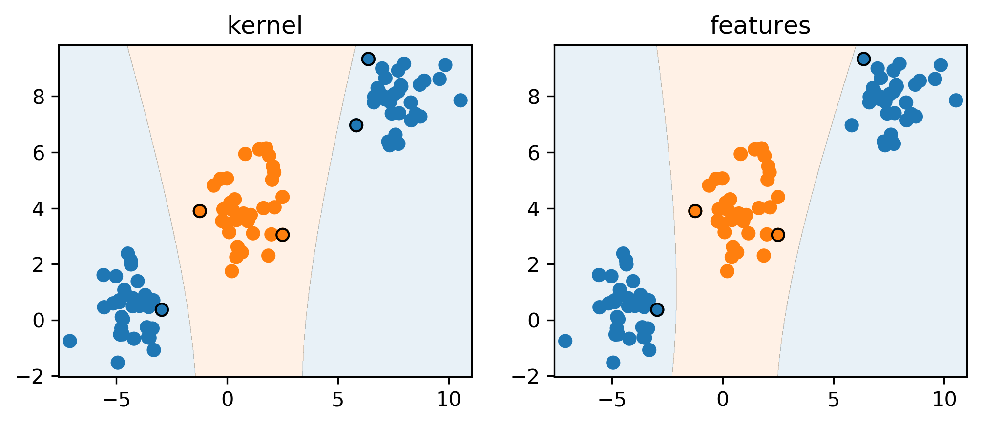
You can see that they’re very similar, by just applying them scikit-learn, either the Kernel SVM or the explicit polynomial features. Here I have this dataset consisting of classes orange and blue. These are not linearly separable. So if I use a linear SVM, it wouldn’t work. But I can do a polynomial transformation to go from two features to five features. In here I just added degree two features. And then I can learn linear SVM on top of these expanded features space. I get a very similar result if I instead of expanding the features, I use the original dataset. But now instead of learning linear SVM, I use a SVM with the polynomial kernel of degree 2, they’re not exactly the same because there was this factor of squared of two that I mentioned, but they’re pretty much the same. Question is if we increase the capacity of the model and we overfit and we’ll talk about this in a little bit, but so, for now, we want to increase the capacity of a model making more flexible I mean, we definitely don’t want to increase it infinitely. But we really making out model more flexible. So here for the polynomial kernel, you could get the same result just by expanding. If you have a very high degree polynomial it would be a large expansion. If you use one of the other kernels, for example, the RVF kernel doing this expansion would actually be resolved in infinite dimensional vector, so you couldn’t actually do this with a feature vector. Now I’m looking at this model here on the right-hand side where I’m using the polynomial features.
Understanding Dual Coefficients
linear_svm.coef_
array([[0.139, 0.06, -0.201, 0.048, 0.019]])
linear_svm.dual_coef_
#array([[-0.03, -0.003, 0.003, 0.03]])
linear_svm.support_
#array([1,26,42,62], dtype=int32)
.smallest[ \($ y = \text{sign}(-0.03 \phi(\mathbf{x}_1)^T \phi(x) - 0.003 \phi(\mathbf{x}_{26})^T \phi(\mathbf{x}) +0.003 \phi(\mathbf{x}_{42})^T \phi(\mathbf{x}) + 0.03 \phi(\mathbf{x}_{62})^T \phi(\mathbf{x})) $\) ]
FIXME formula goes over And so if I look at the linear SVM and I have five coefficients corresponding to the five features. And so if I make a prediction, its first coefficient times the first feature, second coefficient times the second feature and so on, and I look at the sine of it. This is just a linear prediction if I want to look what this looks like in terms of dual coefficients, I can look at the dual coefficients of linear SVM and the support. Out of these many data points, there’s four, they were selected as support vectors by the optimization. These are the ones that have these black circles around them. And so the solution can be expressed as a linear combination of these four support vectors where the coefficients are dual coefficients.
If I want to express this in terms of dual coefficients, I can say its dual coefficient -0.03 times the inner product of the first data point and my test data point in feature space. I do the same thing for the train each point 26 and 42 and 63 with their respective weights. Now I can look at how does this look like for kernel.
With Kernel
poly_svm.dual_coef_
## array([[-0.057, -0. , -0.012, 0.008, 0.062]])
poly_svm.support_
## array([1,26,41,42,62], dtype=int32)
So for kernel, the prediction is this. For kernel SVM there are no coefficients in the original space, there’s only dual coefficients. For each of support vectors, I compute the kernel of support vector with the test point for which I want to make a prediction. This is basically the prediction function of the kernel support vector machine. And you can see it’s very similar to this only that I’ve replaced these inner products by the kernels. The original idea behind this kernel trick was to make computation faster. In some cases, it might be faster.
Runtime Considerations
.center[
 ]
]
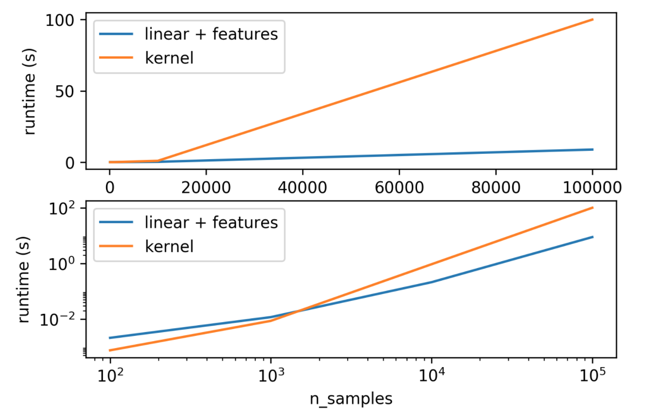
So how does it look like in terms of runtime, here I have the same plot in linear space and log-log space. This is for a fixed number of features, more features make the kernel better. But if I fix the number of features, you can see which of the two is faster. Log-log space is better for this. So you can see that if I have a very small number of samples, then linear kernel and doing explicit polynomials is slower than doing the kernel because of the matrix that’s number of samples times the number of samples is very small. But if I have a lot of features, then doing the explicit expansion is faster since the number of samples is large. In the case where we can do explicit feature expansion if we have a lot of samples, maybe that’s faster.
Kernels in Practice
Dual coefficients less interpretable
Long runtime for “large” datasets (100k samples)
Real power in infinite-dimensional spaces: rbf!
Rbf is “universal kernel” - can learn (aka overfit) anything.
So what does this mean for us in practice? One issue is that the dual coefficients are usually less interpretable because they give you like weightings of inner products with the training data points which is maybe less intuitive than looking at like five times x squared and if you have large data sets they can become very slow. The real power of kernels is when the feature space would actually be infinite-dimensional. The RBF kernel is called the universal kernel, which means you can learn any possible concept or you can overfit any possible concept. Same is true for like neural networks and trees and nearest neighbors, for example, they can learn anything but linear models and even polynomial models of a fixed degree cannot learn everything.
#Preprocessing
Kernel use inner products or distances.
StandardScaler or MinMaxScaler ftw
Gamma parameter in RBF directly relates to scaling of data and n_features – the default is
1/(X.var() * n_features)
Nearly all of these kernels use the distance in the original space. These inner products are distances and so scaling is really important. People use a center scale or min-max scalar.
For the RBF kernel or for any of the kernels really the default parameters work well for scale data. If you don’t scale your data default parameters will not work at all. If you multiply that by five then the default parameters will give you terrible results.
Parameters for RBF Kernels
Regularization parameter C is limit on alphas (for any kernel)
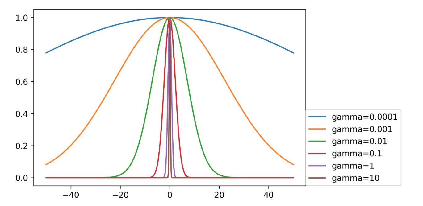
Gamma is bandwidth: \(k_\text{rbf}(\mathbf{x}, \mathbf{x}') = \exp(-\gamma||\mathbf{x} -\mathbf{x}'||^2)\)
.center[
 ]
]
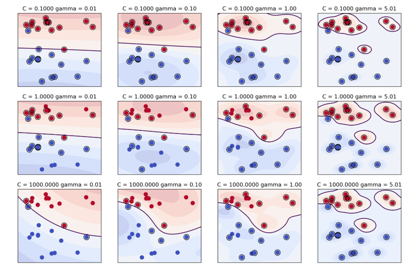
Support vector machine with RBF kernel has these two parameters you need to tune. These both control complexity in some way. We already said that the C parameter limits the influence of each individual data point and the other one is to kernel bandwidth gamma. A smaller gamma means a wider kernel. So wider kernel means a simpler model because the decision boundary will be smoother. Whereas a larger gamma means a much narrower kernel and that means each data point will have much more local influence, which means it’s more like the nearest neighbor algorithm and has more complexity. Usually, you should tune both of these parameters to get a good tradeoff between fitting and generalization.
.center[
 ]
]
This plot tries to illustrate these two parameters in the RBF SVM kernel. On the vertical is C and on the horizontal is gamma and support vectors are marked with circles. So the simplest model is basically the one with the smallest gamma and smallest C. Basically, all data points are support vectors, everything gets averaged and have a very broad kernel. Now, if I increase C, I overfit the data more, each data point can have more influence. And so only the data points that are really close to the boundary have influence now. If you increase gamma, the area of influence of each data point sort of shrinks. So here from it being basically linear or having this very little curvature if you increase gamma, it gets more and more curvature. And in the end, if you make gamma very large, each data point basically has a small sort of isolated island of its class around it giving a very complicated decision boundary. So here, for example, these clearly overfit the training data and so this is probably too large gamma. There’s sort of a tradeoff between the two. Usually, they’re multiple combinations of C and gamma that will give you similarly good results.
from sklearn.datasets import load_digits
digits = load_digits()
.center[
 ]
]
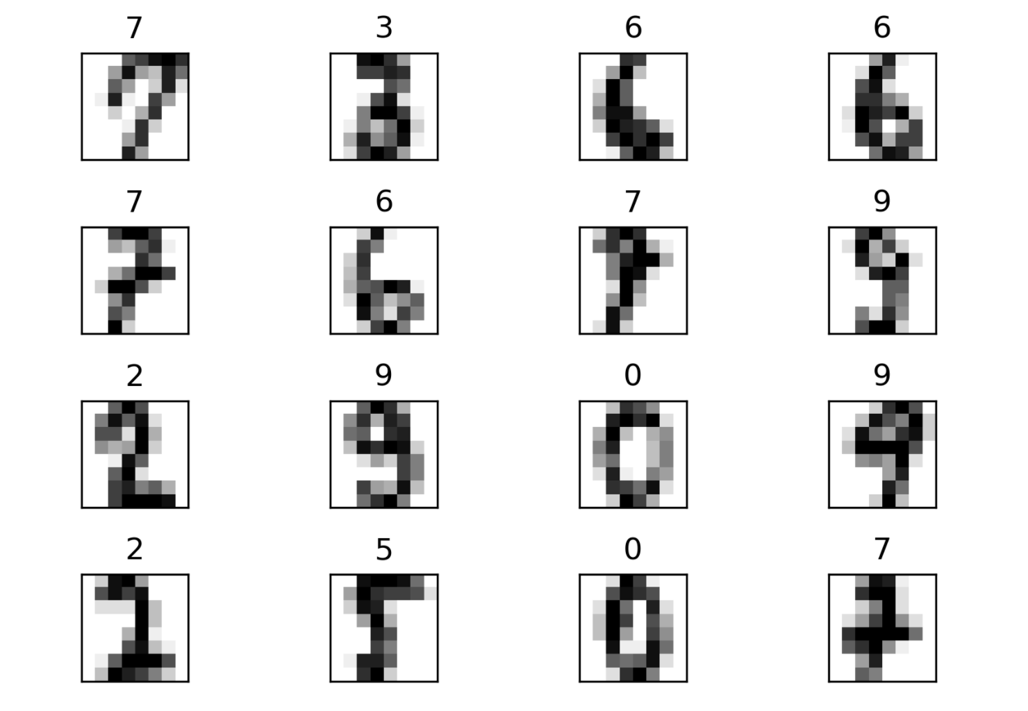
Looking at the digit dataset. Let’s say we want to learn kernel support vector machine on this dataset. So set the two important parameters to tune is C and gamma.
Scaling and Default Params
.smaller[
gamma : {‘scale’, ‘auto’} or float, optional (default=’scale’)
  Kernel coefficient for 'rbf', 'poly' and 'sigmoid'.
  if gamma='scale' (default) is passed then it uses 1 / (n_features * X.var())
  as value of gamma
  if ‘auto’, uses 1 / n_features.
print('auto', np.mean(cross_val_score(SVC(gamma='auto'), X_train, y_train, cv=10)))
print('scale', np.mean(cross_val_score(SVC(gamma='scale'), X_train, y_train, cv=10)))
scaled_svc = make_pipeline(StandardScaler(), SVC())
print('pipe', np.mean(cross_val_score(scaled_svc, X_train, y_train, cv=10)))
auto 0.563
scale 0.987
pipe 0.977
gamma = (1. / (X_train.shape[1] * X_train.var()))
print(np.mean(cross_val_score(SVC(gamma=gamma), X_train, y_train, cv=10)))
0.987
]
Gamma by default in scikit-learn is one over the number of features. This really makes sense only if you scale the data to have a standard deviation of one, then this is a pretty good default. Here if I compare cross-validation, kernel SVM with default parameters on this dataset versus kernel SVM with the scaled data, the performance is either 57% or 97%. There’s a giant jump between the scaled data and the upscale data. Actually here in this data set, all the pixels are on the same scale more or less, so they all are between 0 and 16. So if we change the gamma to be to take into account the standard deviation of the data set, I actually get pretty good results. This is actually just a very peculiar dataset because I basically I know the scale should be from zero to one when it’s from 0 to 16. So scaling by the overall standard deviation gives me good results here. But in principle day, I want to convey is that gamma scales with the standard deviation of the features. Usually, each of the features has a different standard deviation or a different scale and so you want to use a centered scale to estimate the scale for each feature and bring it to one. And then the default gamma, which is one over number of features will be sort of reasonable.
Grid-Searching Parameters
param_grid = {'svc__C': np.logspace(-3, 2, 6),
              'svc__gamma': np.logspace(-3, 2, 6) / X_train.shape[0]}
param_grid
{'svc_C': array([0.001, 0.01, 0.1, 1., 10.,  100.]),
 'svc_gamma': array([ 0.000001, 0.000007, 0.000074,
                      0.000742, 0.007424, 0.074239])}
grid = GridSearchCV(scaled_svc, param_grid=param_grid, cv=10)
grid.fit(X_train, y_train)
To tune them, I use the scaled SVM and both C and gamma usually learn auto log space, so here I have a log space for C and gamma. I actually divide this by the number of features, I could also just change the range, but as I said, this is sort of something that scales with the number of features and standard deviation. Then I can just do my standard grid searchCV with the two-dimensional parameter grid.
Grid-Searching Parameters
.center[
 ]
]
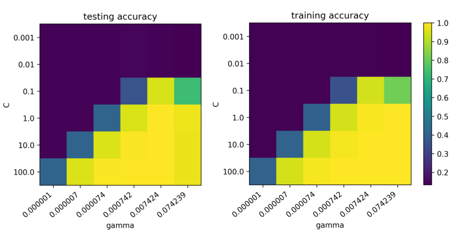
Usually, there’s a strong interaction between these two parameters. And the SVM is pretty sensitive to the setting of these two parameters. So you can see here if you look at the scales, balance 10 classification dataset. So chance performance is 10% accuracy. And so if I set the parameters wrong, I get chance accuracy. If I set them right, I get the high 90s. So that’s the difference between setting gamma to 0.007 and 0.000007 or between setting c to 1 and c to 0.0001.
So usually they’re some correlation between the C and gamma values which are good. So you can decrease or increase C if you decrease gamma and the other way around.
So usually I like to look at grid search results as a 2d heat map for this and if your optimum is somewhere on the boundary, you want to extend your search space. For example, you can see that I wouldn’t need to search this very small Cs, they don’t work at all, but maybe something better might be over here. A C of 100 is already like a very big C so if I want to use even less regularization, learning the model will be even slower.
Questions ?
import matplotlib.pyplot as plt
import numpy as np
import sklearn
sklearn.set_config(print_changed_only=True)
from sklearn.linear_model import Ridge, LinearRegression
from sklearn.model_selection import cross_val_score
from sklearn.datasets import load_boston
boston = load_boston()
X, y = boston.data, boston.target
print(boston.DESCR)
X.shape
fig, axes = plt.subplots(3, 5, figsize=(20, 10))
for i, ax in enumerate(axes.ravel()):
    if i > 12:
        ax.set_visible(False)
        continue
    ax.plot(X[:, i], y, 'o', alpha=.5)
    ax.set_title("{}: {}".format(i, boston.feature_names[i]))
    ax.set_ylabel("MEDV")
print(X.shape)
print(y.shape)
from sklearn.model_selection import train_test_split
X_train, X_test, y_train, y_test = train_test_split(
    X, y, random_state=42)
np.mean(cross_val_score(LinearRegression(),
                        X_train, y_train, cv=10))
np.mean(cross_val_score(
        Ridge(), X_train, y_train, cv=10))
from sklearn.model_selection import GridSearchCV
param_grid = {'alpha': np.logspace(-3, 3, 14)}
print(param_grid)
grid = GridSearchCV(Ridge(), param_grid, cv=10, return_train_score=True)
grid.fit(X_train, y_train)
import pandas as pd
plt.figure(dpi=200)
results = pd.DataFrame(grid.cv_results_)
results.plot('param_alpha', 'mean_train_score', ax=plt.gca())
results.plot('param_alpha', 'mean_test_score', ax=plt.gca())

plt.legend()
plt.xscale("log")
from sklearn.preprocessing import PolynomialFeatures, scale
# being lazy and not really doing things properly whoops
X_poly = PolynomialFeatures(include_bias=False).fit_transform(scale(X))
print(X_poly.shape)
X_train, X_test, y_train, y_test = train_test_split(X_poly, y, random_state=42)
np.mean(cross_val_score(LinearRegression(),
                        X_train, y_train, cv=10))
np.mean(cross_val_score(Ridge(),
                        X_train, y_train, cv=10))
grid = GridSearchCV(Ridge(), param_grid, cv=10, return_train_score=True)
grid.fit(X_train, y_train)
results = pd.DataFrame(grid.cv_results_)

results.plot('param_alpha', 'mean_train_score', ax=plt.gca())
results.plot('param_alpha', 'mean_test_score', ax=plt.gca())
plt.legend()
plt.xscale("log")
print(grid.best_params_)
print(grid.best_score_)
lr = LinearRegression().fit(X_train, y_train)
plt.scatter(range(X_poly.shape[1]), lr.coef_, c=np.sign(lr.coef_), cmap="bwr_r")
ridge = grid.best_estimator_
plt.scatter(range(X_poly.shape[1]), ridge.coef_, c=np.sign(ridge.coef_), cmap="bwr_r")
ridge100 = Ridge(alpha=100).fit(X_train, y_train)
ridge1 = Ridge(alpha=1).fit(X_train, y_train)
plt.figure(figsize=(8, 4))

plt.plot(ridge1.coef_, 'o', label="alpha=1")
plt.plot(ridge.coef_, 'o', label="alpha=14")
plt.plot(ridge100.coef_, 'o', label="alpha=100")
plt.legend()
from sklearn.linear_model import Lasso

lasso = Lasso().fit(X_train, y_train)
print("Training set score: {:.2f}".format(lasso.score(X_train, y_train)))
print("Test set score: {:.2f}".format(lasso.score(X_test, y_test)))
print("Number of features used:", np.sum(lasso.coef_ != 0))
Exercise
Load the diabetes dataset using sklearn.datasets.load_diabetes. Apply LinearRegression, Ridge and Lasso and visualize the coefficients. Try polynomial features.
# %load solutions/linear_models_diabetes.py
