Random Forests
Ensemble Models
One way to get rid of these problems is to actually use multiple trees and Ensemble. Ensemble is a general term that captures any way you combine multiple models into one. There’s like a lot of different kinds of ensemble models that work in many different ways. We’re going to talk particularly about random forest. But that’s only one association of this more general framework.
Poor man’s ensembles
Build different models
Average the result
Owen Zhang (long time kaggle 1st): build XGBoosting models with different random seeds.
More models are better – if they are not correlated.
Also works with neural networks
You can average any models as long as they provide calibrated (“good”) probabilities.
Scikit-learn: VotingClassifier hard and soft voting
If you do computation, we’ll see poor man’s ensembles which is just build the same model multiple times with different random seeds and average them.
Owen Zhang who used to be in the first place in kaggle for five years, he just builds XGBoost models, which are off the tree based models with different random seeds, and then he just averaged all of them. And if you averaged multiple good models, it will get better. This is ideal for competitions.
These are not usually done in practice because it makes the model hard to understand, it takes more RAM, it takes more time to predict because you have to do it like number of models many times.
In scikit-learn, there’s this voting classifier which just takes the list of models of different types or be the same model type with different visualizations. And it will train all of them and average the results.
You can either do soft voting or hard voting. Soft voting means averaging the probabilities and take the arg max. Hard voting means everything makes a prediction and then you take the thing that was most commonly predicted.
VotingClassifier
.smaller[
voting = VotingClassifier(
    [('logreg', LogisticRegression(C=100)),
     ('tree', DecisionTreeClassifier(max_depth=3, random_state=0))],
    voting='soft')
voting.fit(X_train, y_train)
lr, tree = voting.estimators_
tree.score(X_test, y_test), lr.score(X_test, y_test), voting.score(X_test, y_test)
0.80 0.84 0.88
]
.center[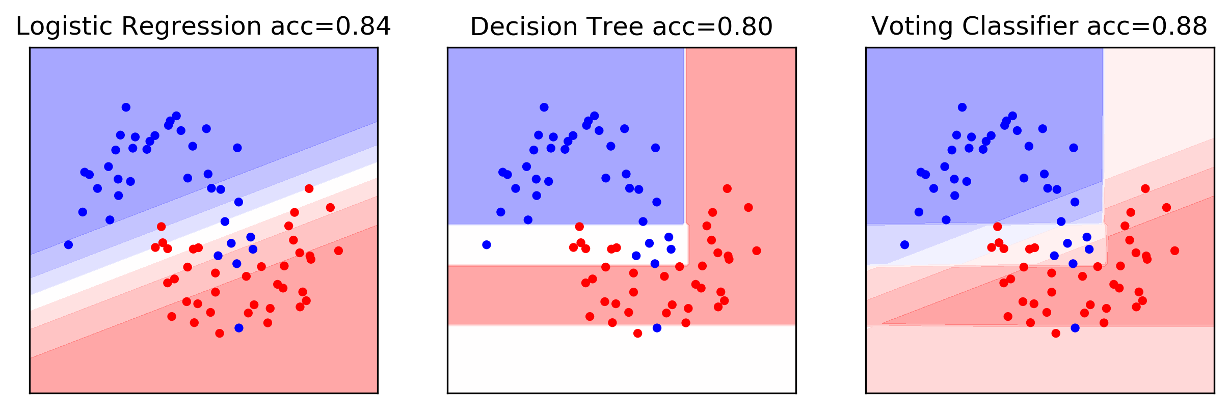 ]
]
It looks like this. Here is the logistic regression model on this 2D data set. This is the decision tree based model and the voting classifier weights - probability estimates by most of them. And if you want, you can do that. Again, mostly done in competitions.
The easiest way to do ensembles is to just average models. Problem is, if they overfit in the same way, you’re not going to get rid of the overfitting. So what you really want to do is you want to make sure you have models that are quite different from each other and you averaged the models that are different.
Bagging (Bootstrap AGGregation)
.left-column[
Generic way to build “slightly different” models
BaggingClassifier, BaggingRegressor ] .right-column[ .center[
 ]
]
]
]
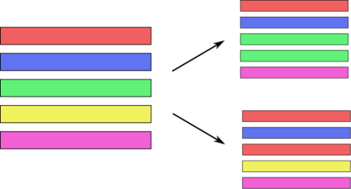
One way to do this is called Bagging or Bootstrap Aggregation. And the idea in bagging is, imagine that these are your data points, you have five data points and so you want to make sure that you built similar but slightly different models. And you want to do more than just change the random seed. One way is to take bootstrap samples of your dataset. Bootstrap samples mean sampling with replacement, number of samples many points. So here in this example, from these five data points, I would sample a new dataset that again has five data points (sample with replacement). On average this will mean that each dataset will have about 66% of the original data points, and the other data points will be just duplicates. So you leave out some data, duplicate some other data, and you end up with a slightly different dataset.
You can do this obviously, as often as you want. If you average these models, if the model was prone to overfitting, then the average might not overfit as much.
Draw bootstrap samples from dataset
(as many as there are in the dataset, with repetition)
Bias and Variance
.center[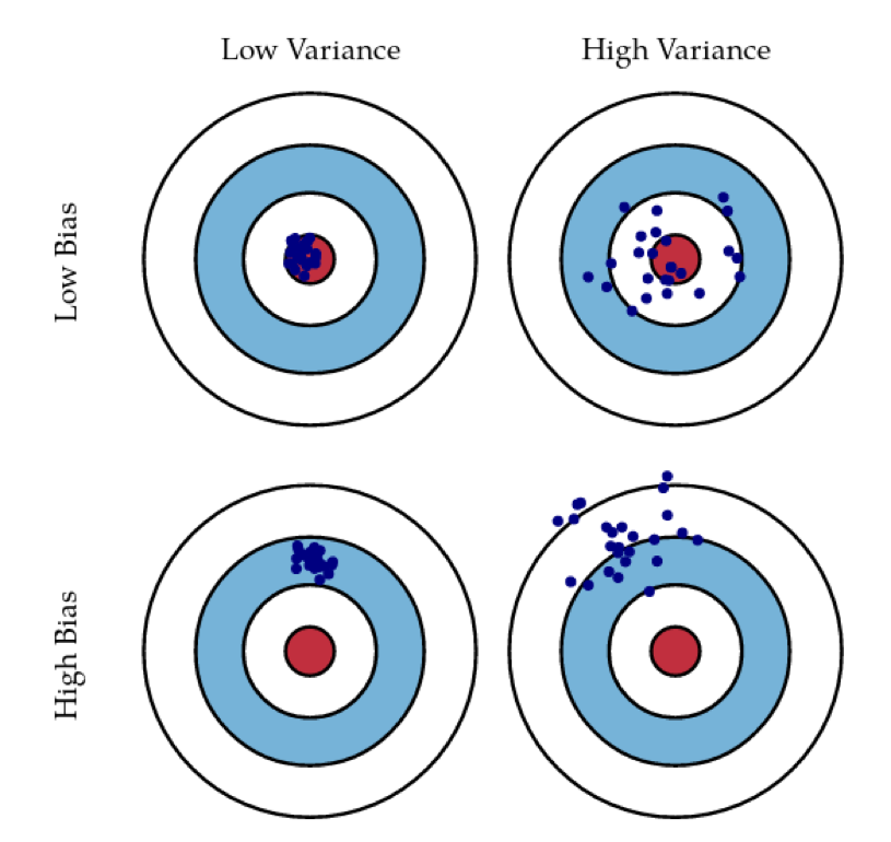 ]
]
.left[ .smaller[http://scott.fortmann-roe.com/docs/BiasVariance.html] ]
What you often hear in this context is talking about bias and variance, which is not entirely the same thing as underfitting and overfitting but quite related to it. The idea is that the errors you make on the test set are basically combinations of the error you make in modeling plus the uncertainty in the modeling.
The idea is that you can have models that are very consistent, but off. So that would be a high bias low variance model. So this would be, for example, a low dimensional linear model that is mixed inconsistent predictions, but it might not be able to capture the target very well since it’s not powerful enough.
You want ideally a model that has low bias and low variance. So that’s sort of captures the data concept very well and also has very little variance in the predictions it makes. A high variance model is one that on average captures the predictions but has very high variance in the prediction it makes.
The idea of bagging is that you can take multiple high variance models and if you average them, then it will reduce the variance of the average. If the predictions are not very correlated, then there’s like a very nice, easy proof to say that if I average multiple high variance estimators, I get a low variance estimator.
They need to be sort of good enough, on average, if they’re all really, really bad, and if you average then it will still be pretty bad.
Bias and Variance in Ensembles
Breiman showed that generalization depends on strength of the individual classifiers and (inversely) on their correlation
Uncorrelating them might help, even at the expense of strength
There’s this proof that shows that if you have decorrelated errors, then averaging will help. Basically, the correlation between the errors that you make shows up there. And so the idea is to make the errors as different as possible. Maybe even go further than the bagging in trying to make sure the different models that you build are as different from each other as possible, while still being reasonably good models. This leads to the idea of random forests, which basically tries to randomize trees, even more than you would do with bagging, and then average results of these trees.
FIXME worst slide!
Random Forests
.center[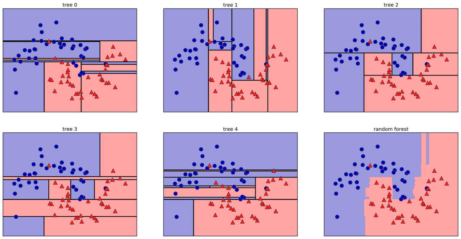 ]
]
Here example of a random forest on a 2-dimensional dataset.
Smarter bagging for trees!
Randomize in two ways
.left-column[
For each tree:
Pick bootstrap sample of data
For each split:
Pick random sample of features
More trees are always better ]
.right-column[

 ]
]
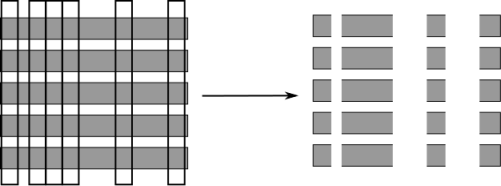
The way that random forest work is they randomize tree building in two ways. As with bagging if you do a bootstrap sample of the dataset, so each tree you take a bootstrap sample of the data set and then for each split in the tree, you take a sampling without replacement of the features. So let’s say you have this representation of the dataset again. And for each node where you want to make a splitting decision before you want to scan all over the features and all the thresholds, you select just the subset of the number of features and just look for splits there. And this is done for each node independently. In the end, the tree will use all the features probably, if it’s deep enough, eventually it might use all the features but you randomize the tree building process in a way that hopefully de-correlated the error of the different trees. And so this adds another hyperparameter in the tree building.
Tuning Random Forests
Main parameter: max_features
around sqrt(n_features) for classification
Around n_features for regression
n_estimators > 100
Prepruning might help, definitely helps with model size!
max_depth, max_leaf_nodes, min_samples_split again
Which are max features, which is the number of features that you want to look at each split. So the heuristic is usually for classification you want something like the square root of the number of features, whereas, for regression, you usually want something that is around the same size as the number of features. This basically, controls the variance of the model because if you set this to number of features, it will be just sort of the old decision tree. If you set this to one, it will pick a feature at random, and then it needs to split on that feature, basically.
So this will be like a very, very random tree that probably would grow very deep because it can really make good decisions.
This is the main parameter that you need to tune, although random forest is actually very robust to these parameter settings. Usually, if you leave this to the default, it will be reasonably well.
By default, in scikit-learn, the number of trees in the forest is way too low. Usually, you want something like 100, or 500 but scikit-learn only gives you like 10.
Sometimes people find that pre-pruning techniques like maximum depth or maximum leaf nodes help. Generally, the idea doesn’t really matter that much, how good the vigil trees are as long as you have enough of them. But limiting the size of the tree will definitely help with model size. That said, if you randomize a lot, these trees will grow very deep. Because if you’re unlucky, you’ll always just split on bad feature so you will always not really get much further in getting pure leaves and so you need to do a lot of splits. So setting something like max depth will allow you to decrease RAM size and decrease prediction time.
Extremely Randomized Trees
More randomness!
Randomly draw threshold for each feature!
Doesn’t use bootstrap
Faster because no sorting / searching
Can have smoother boundaries
Alright, so there’s a slightly different variant of random forest that’s also kind of interesting, which is Extremely Randomized Trees. They work very similarly except for the fact that you draw randomly a threshold for each feature. So here, you don’t search over the thresholds, you just pick one at random. And usually, you don’t use bootstrap.
Since you don’t need to do sorting these are faster to build. You probably get smoother decision boundaries since the thresholds are drawn at random.
Sometimes they aren’t as bad as random forest but they’re definitely not commonly used as the default random forest.
One of the nice things about extremely randomized trees and the random forests is they work without any preprocessing. If you set number of estimators large enough, they will just work. They will not be the best model but they will always work.
Warm-Starts
.smaller[
train_scores = []
test_scores = []

rf = RandomForestClassifier(warm_start=True)
estimator_range = range(1, 100, 5)
for n_estimators in estimator_range:
    rf.n_estimators = n_estimators
    rf.fit(X_train, y_train)
    train_scores.append(rf.score(X_train, y_train))
    test_scores.append(rf.score(X_test, y_test))
]
.center[
 ]
]
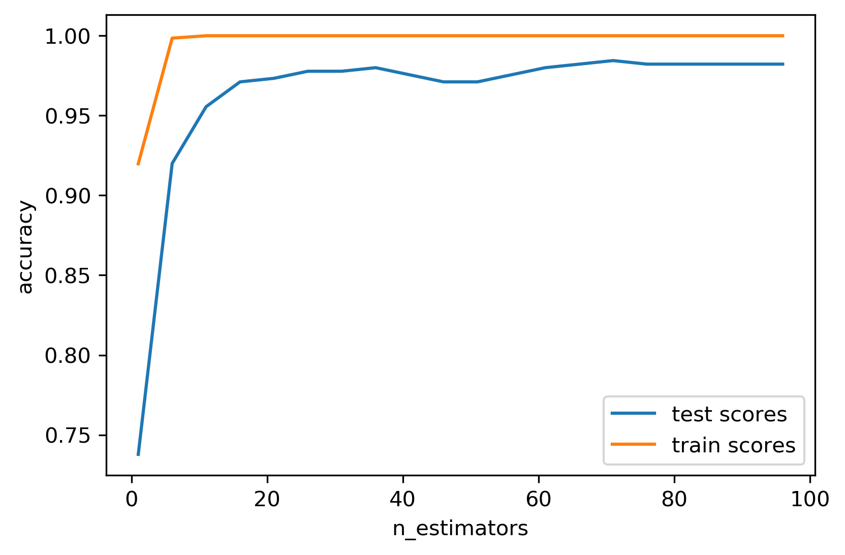
The more trees you use, the better it is since you decrease the variance more. Don’t ever grid search the number of trees, because the higher will be better and you’re just wasting your time.
But there are diminishing returns. So maybe 100 trees are good enough and if you built 500 trees, again, you’re wasting your time and you might not want to do that.
In scikit-learn, when you use Warm-Starts, you basically iteratively add more and more trees to the forest and you can stop whenever you think it’s good enough.
Basically, the fit method will keep all the previous trees and add on more trees.
I go from 1 feature to 100 features in steps of five. I set the number estimator. So I started with one tree and then increased by five every time. I fit the model. And then I look at training and test score. This is much better than grid searching it because in grid search I would do the same work over and over again, while here, I’m adding more and more trees and find out what is it good enough.
Usually, I would double the search like 50, 100, and 200 and so on and find where it stabilizes, and then only I will stop adding more trees.
If you don’t want to do that, just picking large enough number and stick to that number. Then you don’t need to fiddle around as much but you might be wasting computational resources that could be used otherwise for like parameter tuning, for example.
Out-of-bag estimates
Each tree only uses ~66% of data
Can evaluate it on the rest!
Make predictions for out-of-bag, average, score.
Each prediction is an average over different subset of trees
.smaller[
train_scores = []
test_scores = []
oob_scores = []

feature_range = range(1, 64, 5)
for max_features in feature_range:
    rf = RandomForestClassifier(max_features=max_features, oob_score=True,
                                n_estimators=200, random_state=0)
    rf.fit(X_train, y_train)
    train_scores.append(rf.score(X_train, y_train))
    test_scores.append(rf.score(X_test, y_test))
    oob_scores.append(rf.oob_score_)
]
Another thing is looking at out of back estimates. This is something that’s specific to random forest. That said, if you do bootstrap sampling, usually you get like 66% of your data for each estimator. That means there’s about 33% of your data that you haven’t used for each individual tree. So you can use that data as a test set for that particular tree.
The out of back estimate in a random forest is for each tree, I individually predict on the 33% on which I haven’t trained. And then for each data point, I look at all the trees that held out this particular data point and let them vote. So then for each data point, I only have a subset of the trees that makes a prediction but if I have enough trees overall, it’ll still be fine.
Let’s say, I used 300 estimators, then basically, on average, for each data point, I will have 100 estimators that didn’t use those data points. And so it can use this data point as a test set for this 100 estimators and can let them vote on what the prediction should be. And this way, basically, I get a test set score for free. In fact, it’s like a bootstrap estimate of a test set score.
And so basically, I don’t need to use a test set, I can just use the out of bag estimate.
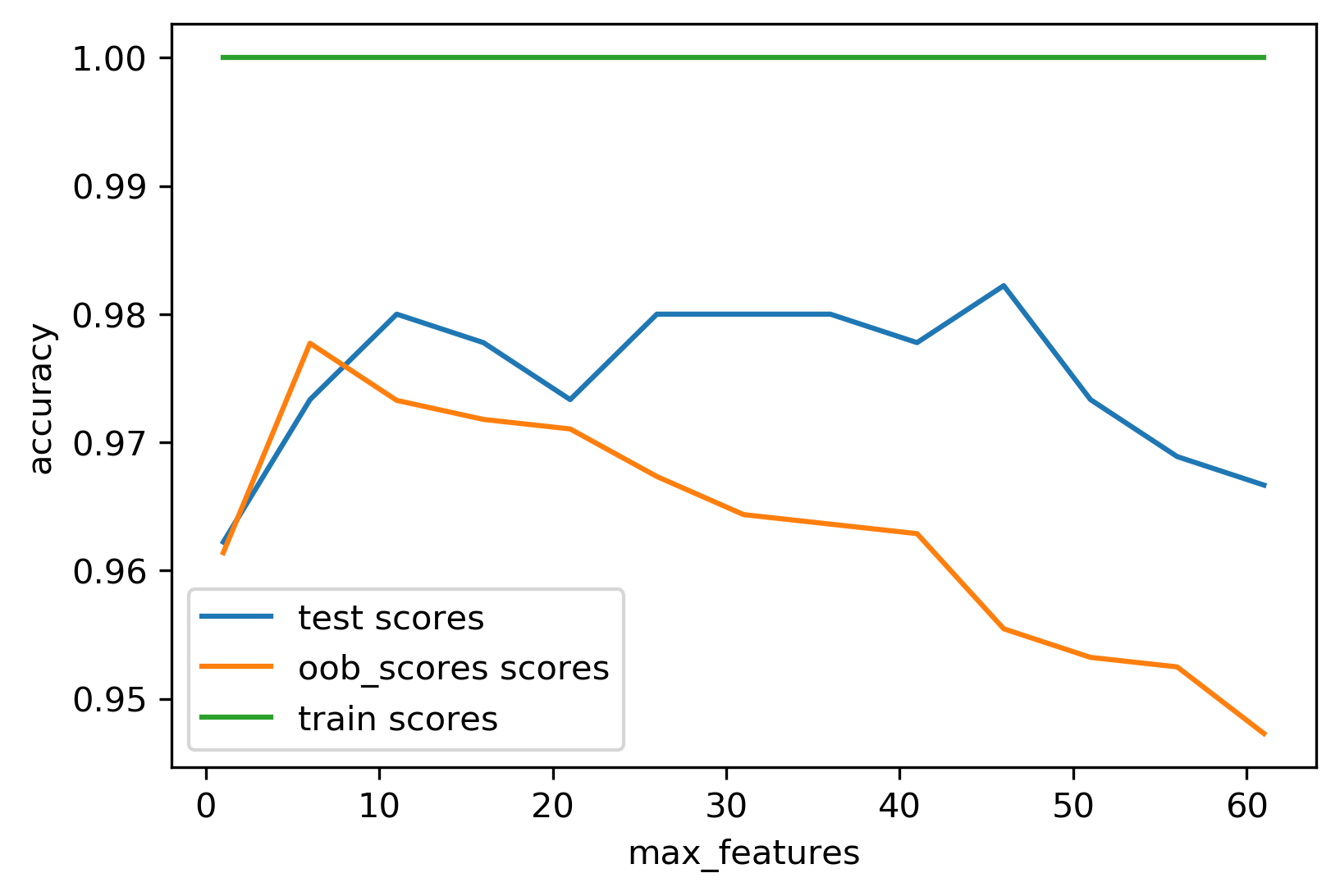
So here, for example, using this to find the best number of features. I look for max number of features in a particular range in a random forest classifier. In this case, for illustration purposes, I use both the out of bag estimate and the test set scores to see how they compare.
.center[
 ]
]
You can see that since I didn’t prune the trees in any way, the training scores is always one because it’s always perfect and you perfectly overfit everything. The test sets scores and the out of bag scores are at least somewhat similar in trend and also in magnitude because the out of bag estimate uses only one-third of the trees, it might be slightly worse. But basically, I got this for free without spending any additional data or any additional computation.
And so both of these probably have a habit of uncertainty. I have no uncertainty estimate but theoretically, this is sort of an unbiased estimate of the test set accuracy.
Variable Importance
.smaller[
X_train, X_test, y_train, y_test = train_test_split(
    iris.data, iris.target, stratify=iris.target, random_state=1)
rf = RandomForestClassifier().fit(X_train, y_train)
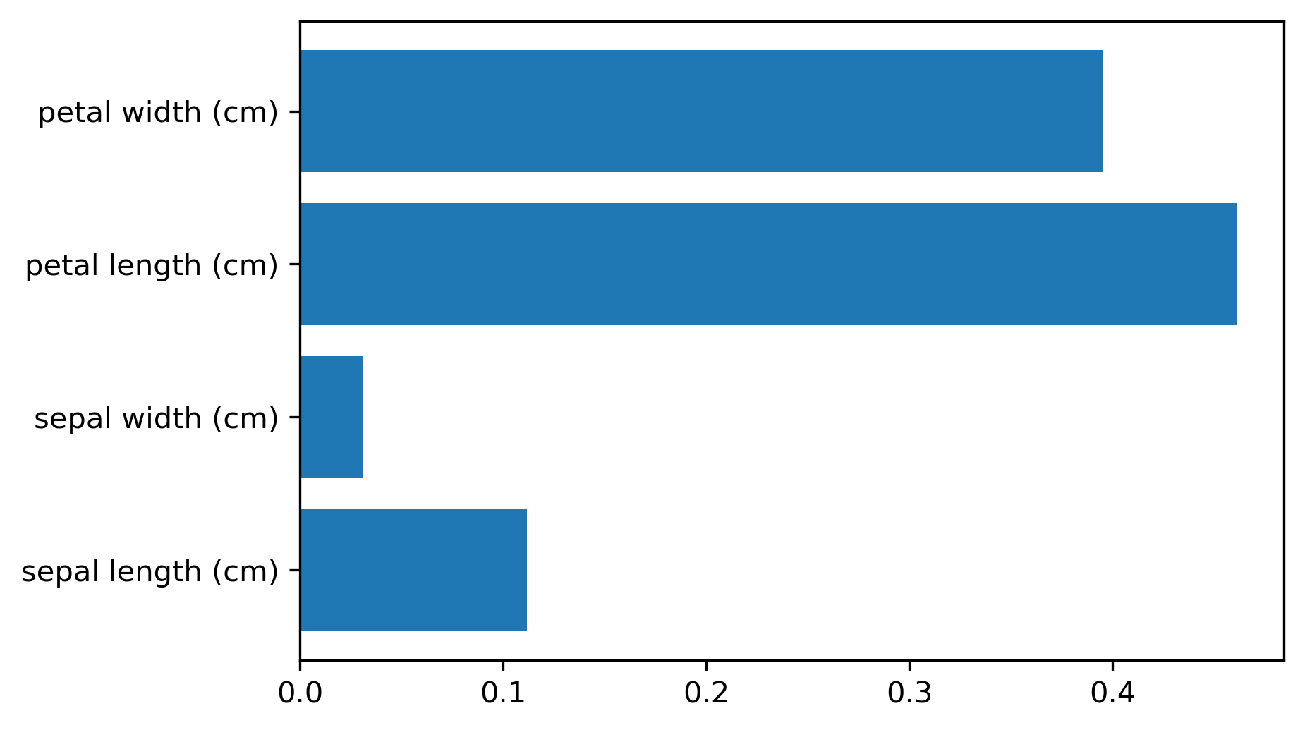
rf.feature_importances_
plt.barh(range(4), rf.feature_importances_)
plt.yticks(range(4), iris.feature_names);
array([ 0.126, 0.033, 0.445, 0.396])
]
.center[
 ]
]
As for the trees, for the random forest, I can get variable importance. And these are more useful now because they’re more robust. Again, they don’t have directionality.
But now, if you have two correlated features, probably if you build enough trees, and because of the way they’re randomized, both of these features will be picked some of the time. And so if you average over all of the trees, then both will have the same amount of importance. So this will basically just give you like a smoother estimate of the feature importance that will be more robust and will not fail on correlated features.
Questions ?
Question: Is there a statistical test where the variable is important?
It’s probably the wrong question to ask. Because these are like greedily trained and so trying to extract any statistical meaning out of that is probably not the best idea. So if you’re trying to understand your dataset or your data generating process, I probably wouldn’t use tree-based models. These are really good for predicting no matter what your input is.
Question: How is the feature importance calculated?
Whenever a particular feature was used in the tree, you look at the decrease in impurity, and you aggregate these and at the end, you normalize it sum to one.
import numpy as np
import matplotlib.pyplot as plt
import sklearn
sklearn.set_config(print_changed_only=True)
import pandas as pd
from sklearn.model_selection import train_test_split
from sklearn.pipeline import make_pipeline
from sklearn.preprocessing import scale, StandardScaler
from sklearn.datasets import load_breast_cancer
cancer = load_breast_cancer()
print(cancer.DESCR)
X_train, X_test, y_train, y_test = train_test_split(
    cancer.data, cancer.target, stratify=cancer.target, random_state=0)
tree visualization
from sklearn.tree import DecisionTreeClassifier, plot_tree
tree = DecisionTreeClassifier(max_depth=2)
tree.fit(X_train, y_train)
plt.figure(dpi=200)
plot_tree(tree, feature_names=cancer.feature_names, filled=True)
Parameter Tuning
tree = DecisionTreeClassifier().fit(X_train, y_train)
plt.figure(figsize=(15, 5))
plot_tree(tree, feature_names=cancer.feature_names, filled=True)
tree = DecisionTreeClassifier(max_depth=3).fit(X_train, y_train)
plt.figure(figsize=(15, 5))
plot_tree(tree, feature_names=cancer.feature_names, filled=True)
tree = DecisionTreeClassifier(max_leaf_nodes=8).fit(X_train, y_train)
plot_tree(tree, feature_names=cancer.feature_names, filled=True)
tree = DecisionTreeClassifier(min_samples_split=50).fit(X_train, y_train)
plot_tree(tree, feature_names=cancer.feature_names, filled=True)
tree = DecisionTreeClassifier(min_impurity_decrease=.01).fit(X_train, y_train)
plot_tree(tree, feature_names=cancer.feature_names, filled=True)
from sklearn.model_selection import GridSearchCV
param_grid = {'max_depth':range(1, 7)}
grid = GridSearchCV(DecisionTreeClassifier(random_state=0), param_grid=param_grid, cv=10)
grid.fit(X_train, y_train)
from sklearn.model_selection import GridSearchCV, StratifiedShuffleSplit
param_grid = {'max_depth':range(1, 7)}
grid = GridSearchCV(DecisionTreeClassifier(random_state=0), param_grid=param_grid,
                    cv=StratifiedShuffleSplit(100), return_train_score=True)
grid.fit(X_train, y_train)
scores = pd.DataFrame(grid.cv_results_)
scores.plot(x='param_max_depth', y=['mean_train_score', 'mean_test_score'], ax=plt.gca())
plt.legend(loc=(1, 0))
from sklearn.model_selection import GridSearchCV
param_grid = {'max_leaf_nodes': range(2, 20)}
grid = GridSearchCV(DecisionTreeClassifier(random_state=0), param_grid=param_grid,
                    cv=StratifiedShuffleSplit(100, random_state=1),
                   return_train_score=True)
grid.fit(X_train, y_train)

scores = pd.DataFrame(grid.cv_results_)
scores.plot(x='param_max_leaf_nodes', y=['mean_train_score', 'mean_test_score'], ax=plt.gca())
plt.legend(loc=(1, 0))
scores = pd.DataFrame(grid.cv_results_)
scores.plot(x='param_max_leaf_nodes', y='mean_train_score', yerr='std_train_score', ax=plt.gca())
scores.plot(x='param_max_leaf_nodes', y='mean_test_score', yerr='std_test_score', ax=plt.gca())
grid.best_params_
plot_tree(grid.best_estimator_, feature_names=cancer.feature_names, filled=True)
pd.Series(grid.best_estimator_.feature_importances_,
          index=cancer.feature_names).plot(kind="barh")
Exercise
Apply a decision tree to the “adult” dataset and visualize it.
Tune parameters with grid-search; try at least max_leaf_nodes and max_depth, but separately.
Visualize the resulting tree and it’s feature importances.
